Population Bomb: Forecast Gone Wrong?

Today the New York Times published a Retro Report titled The Unrealized Horrors of Population Explosion accompanied by the video above. The report takes a look at predictions made by American biologist Paul Ehrlich in his 1968 book The Population Bomb. In the book, Ehrlich presented future scenarios (he clearly stated they weren't predictions) that, for example, by 1970 hundreds of millions of people would starve from population growth increasing faster than food production (basically a restatement of the Malthusian Catastrophe). It didn't happen and, regardless of Ehrlich's protestations, his "predictions" have come to be viewed as notorious examples of forecasts that proved wrong. But more is at stake here than Ehrlich's forecasting ability.

Population growth is the primary exogenous forcing variable in the IPCC Emission Scenarios, in Limits to Growth Models and in Neoclassical Economic Growth Models that do not recognize any limit to growth (see my discussion here). If Ehrlich's predictions were wrong does that mean that there are no limits to growth and that we don't have to worry about CO2 emissions? I'll let you watch the video, read the New York Times article, follow the other links and think about this question.

In future posts, I'll make my own forecasts for World population and look at what some of the consequences might be.

A More Conservative Peak Oil Forecast

In an earlier post (here) I presented a Peak Oil forecast that was pretty pessimistic: world oil production would collapse by 2040. I have been reluctant to publish this forecast because (1) the conclusions seemed pretty catastrophic and (2) the prediction intervals just looked too good, that is, too narrow implying a high degree of confidence that I didn't have. Above is another Peak Oil forecast with different prediction intervals that seem more realistic, that is, the downturn in world oil production might persist for a while but there is some probability (however small) that new technologies will come along that allow oil production to continue expanding. 

The problem with the original set of prediction intervals is that they did not take into account the error in the WL20 state variables that were used as input variables to the Peak Oil forecast. It was simply assumed that the raw forecast outputs of the WL20 model were the best future predictors for the world system. In any conventional forecasting model that has input variables, it is typically assumed that the forecast input variables are the best future predictors for the system. The assumption is certainly questionable and, at minimum, does not recognize that any model-based forecast has uncertainty attached to its outputs. Here's a simple causal diagram:

Typically, forecasts only take E2 into account when construction a forecast as was done with my initial Peak Oil forecast. E1 is simply ignored even though there is clearly cascading uncertainty in the model.

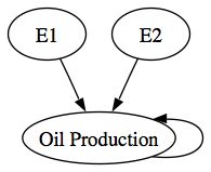
The conservative forecast above essentially takes both the E1 and E2 errors into account when computing prediction intervals for oil production since E1 is transmitted indirectly through the WL20 state variables.

A question at this point would be what if we ignored the E1 path entirely and just predict Oil Production without any input variables, what I would call a business as usual or BAU forecast. The Hubbert curve or Hubbert peak models were essentially BAU models with a different functional form i.e., the Logistic Distribution Curve. The advantage of the BAU models is that there is no cascading uncertainty. The BAU forecast in the graph above predicts that oil production will approach a peak somewhere between 80 million and 140 million tons of oil equivalent and stay there forever. This forecast is probably consistent with the improbable upper prediction interval of our initial conservative forecast.

Aside from the fact that we know oil is a nonrenewable resource, why should we prefer any of these plausible forecasts over any of the others? If we limit ourselves to the step-ahead AIC criteria, the BAU model is the winner with [264.70 < AIC=240.18 < 309.53] compared to the world system model with [290.42< AIC=279.72 <315.11]. However, if instead we calculate the attractor-based AIC, the WL20 model is best with AIC = 278.58 as compared to AIC=538.30 for the random walk model and AIC=315.06 for the BAU model. In other words, the BAU model is good at predicting next year's oil production but not very good at looking 50 years into the future (recall that the attractor simulation starts in 1950 and, from that initial position, simulates oil production out to 2008).

My experience has been that single equation models such as the BAU model or the Logistic model, are good at step-ahead predictions and are not subject to cascading uncertainty from input variables. However, single-equation models are not necessarily very good at predicting into the future even if the confidence intervals look quite narrow. And, because attractor models describe a path the system wants to move toward, their predictions also make more theoretical sense. The key here is to run the attractor simulation and compare the AICs for that simulation rather than the step-ahead simulation.

The ultimate test of all this is to compare the actual path of oil production over the next thirty years to the predictions of the various models--I just won't be around to make that comparison. In the next post, I'll explain how to generate these forecasts for the next generation in case they are interested.

Using Forecasting Models

In an earlier post (here) I explained how to use the WL20 model and the ws (world system) package. In this post, I will explain how to use forecasting models such as the one used to make my Peak Oil forecast (here).

Assuming that you have followed my earlier post, have R installed on your machine and have also installed the dse and the matlab packages successfully, the forecasting models are all available here. For this demonstration, download the PeakOilIndexModel to your working directory. Then you can enter the following commands at the > prompt in the R console:

> W <- "the complete path name for your working directory"

> setwd(W)

> source(file="LibraryLoad.R)

> load(file="WL20v3_model")

> load(file="ws_procedures")

> load(file="PeakOilIndexModel")

The available forecasting models can be seen by typing (a help file for all the ws package functions is available here):

> summary(OIL.model)

The resulting listing will show each of the available models. For example,

[1] "BAU"

Eigenvalues of system matrix

[1] 0.9836614

[1] TRUE

     Parameter     Mean Mean LCI Mean UCI P>=T[1] P< T[1]

[1,]  240.1784 288.4285 264.6985 309.5271       1       0

     Std. Dev.      Bias    Bias-z

[1,]  18.21428 -48.25009 -2.649025

attr(,"class")

[1] "boot"

[1] "STRUCTURAL"

NULL

The BAU (Business As Usual) entry shows a number of statistics used to evaluate the model. The Structural model displays NULL because no structural model was estimated.

The first statistic displayed for the BAU model is the eigenvalue of the system matrix. If all the eigenvalues are less than unity, the model is stable, which is displayed next as [1] TRUE. The next line shows the bootstrap distribution of the AIC statistic. The first value, 240.1784, is the sample AIC statistic. The second value is the bootstrap mean AIC statistic. The third and fourth values are the lower and upper 98% confidence intervals for the AIC statistic. The remaining values display probabilities, standard deviation and bias for the sample AIC statistic. If you want to inspect the BAU model, enter:

> getModel(OIL.model,type="bau")

Given the AIC statistics, the BAU model is the best one observed. For the forecast, however, I used the  best attractor model which you can display with

> getModel(OIL.model,type="best attractor")

The best attractor model is based on a free-simulation of each estimated model and is chosen using the AIC statistic from the free simulations vs. the actual data residuals. In this case, the world index model

> getModel(OIL.model,type="world index")

provides the best attractor simulation. You can get a flavor for the differences in the predictions from the two models by entering:

> tfplot(sim(getModel(OIL.model,type="bau")))

> tfplot(sim(getModel(OIL.model,type="world index"),sampleT=95,input=WL20.fx))

The BAU model predicts a gradual decline over time in the rate of oil production while the best attractor model shows a sharp peak-and-collapse between 2000 and 2020. 

Why should we be willing to choose one of these models over the other? One is best by conventional standards (step-ahead predictions using the AIC). Another is best by standards derived from attractor theory and application of the AIC criteria to the free simulations of each model. 

In future posts, I'll work through this issue and also reveal some more of the things you can do with the forecasting models using the dse and the ws packages. At this point, you should be able to at least load and inspect the models.

Has Smallpox Been Eradicated?

The Earth Policy Institute published today (here) an article on smallpox and polio. Smallpox caught my attention after reading the following quote from the article:

Smallpox plagued humanity for thousands of years. In the 18th century, smallpox killed one out of every ten children in France and Sweden. Over the 20th century, the virus caused between 300 and 500 million deaths worldwide. No effective treatment was ever developed.

The eradication of this devastating disease is one of public health’s greatest achievements. It involved mass vaccinations and surveillance to track and contain outbreaks. In 1977, ten years after the World Health Organization (WHO) began an intensive eradication program, the last naturally occurring case of smallpox was identified in Somalia. And on May 8, 1980, the World Health Assembly declared smallpox eradicated.

What also caught my attention was the large spikes in the number of reported cases after World War II, in the late 1950's and in the mid-1970's. My question was what caused the spikes and whether we could be sure that surveillance and vaccination were enough to prevent future outbreaks.

The result of my forecast from the WL2o model is presented in the graphic above. It suggests that future outbreaks are possible. The reason is that the late 20th century spikes are related to spikes in commodity market prices. Whatever the mechanism, future problems in commodity markets (which can be anticipated based on peak oil forecasts) could have unanticipated population health consequences.

Forecasting During The Great Recession

Tyler Cowen (here) has argued that since we do not have models that describe the current economic crisis, we really won't be able to forecast when the economy will recover (even though many forecasters are currently trying). Cowen makes a reasonable argument and has certainly thrown down the gauntlet to the forecasting community.

There are a group of forecasters led by the notorious J. Scott Armstrong (Armstrong bet Al Gore $10,000 US that future global temperature cold not be predicted--Gore refused the bet) who think the have the forecasting problem solved. The group argues (here) that there are 139 forecasting principles that are used by successful forecasters. Now would be an interesting time to see whether these principles could improve models of the US economy and lead to better forecasts.

Here are a few random thoughts on current approaches to forecasting:

• The focus should be on our existing models. However, I don't agree with Cowen that a model has to explain everything, for example, business confidence or regulatory uncertainty. A simple canonical forecasting model would be Q(t) = a + b Q(t-1) + e(t), the simple difference equation. A lot of forces such as "confidence" and "uncertainty" must fall into the error term, e(t). It's surprising how many forecasts are presented without prediction intervals based on observed error terms.
• The principles approach to forecast is way too ad hoc. If a forecast doesn't work, there's always a violated principle somewhere to explain the failure. One principle. for example, is that some things (like global warming if you believe Prof. Armstrong) cannot be forecast (the perfect escape clause). However, in that case, the model reduces to Q(t) = Q(t-1) + e(t), the random walk. In another blog (here), I'm searching for random walks in the stock market. Contrary to widely held academic opinion (here), finding stocks that are clearly random walks is not that easy.
• These considerations bring us back to the model again and particularly how the error term, e(t), is treated. One explanation for forecasting failure leading up to the Great Recession is that the Recession itself was a black swan event, unusual and improbable given widely held prejudices about normal distribution theory and error terms.
• There are problems with the way forecasts are typically constructed. If we try to predict tomorrow's Q(t) from yesterday's Q(t-1), we have to remember that Q(t-1) is not itself known with certainty. If errors tend to accumulate over time (as in the random walk model), the system may be very far away from reasonable values (as it was in the Subprime Mortgage crisis). In other words, forecasting during a bubble will work fine until the bubble bursts when the forecasts will be quite wrong.

To summarize, I think Tyler Cowen has it backwards. Forecasting right now should be easy. The bubble has burst. Forecasting when the next bubble will develop (a "return to normalcy") is another problem entirely.

Most of these issues are the subject of this blog and will be the topic of future posts.