Climate Uncertainty

Calculating Forecasting Odds: Think Like a Stockbroker

In a Take Part article (here), Amy Luers, Director of Climate Change at the Skoll Global Threats Fund, takes on the issue of variability and forecasting. Leurs makes the argument that global temperature forecasting and stock forecasting have similar problems with statistical variability. Working with Leonard Sklar, Professor of Geology at San Francisco State University, Leurs developed the two graphs above. On the left is the Dow Jones Industrial Average (DJI, my forecast for the SP500 is here), on the right is Global Temperature (my forecast is here). The bottom left graph shows the odds of making money if you invested in any random year (1913-2010) and stayed in the stock market for up to 50 years. After about 35 years of staying invested, there is a 100% chance of making money. On the right is the same graph for global temperature. It takes a little longer, but after 45 years you have a 100% chance of finding a temperature increase. Notice that in both cases, if you look over only brief periods, the odds are closer to 50-50.

The graph above is from page 381 of Nate Silver's book The Signal and the Noise. In 2007, the notorious Scott Armstrong, Professor of Marketing at the Wharton Business School, made a $10,000 bet with Al Gore that Armstrong modestly called "The Global Warming Challenge." Armstrong and his colleague Kesten Green, an Australian Business School Lecturer,  have argued (here) that Global Temperature is too variable to forecast. The Armstrong-Gore bet was to be resolved monthly. Predicting "no-change," Armstrong argued from the data above that he had won the bet.

Given the Luers-Sklar data, we understand why Armstrong made this bet and we also understand why Al Gore never took the bet. Five years is far too short a time to determine whether temperature has increased or whether, for that matter, the stock market has made money. Having published "Principles of Forecasting, [...a book that...] should be considered canonical to anybody who is seriously interested in the field [...of forecasting]" (these are Silver's words), Prof. Armstrong should have known better.

The basic problem with Prof. Armstrong, his "Global Warming Challenge" and his forecasting principles (I have commented on the principles here) is summed up by a quote from Nelson Mandela "Where you stand depends on where you sit" and Prof. Armstrong sits in the business school and is paid to market business activity as having little impact on the environment. All the forecasting principles and outrageous bets in the world will not cover up this canonical conflict.

A More Conservative Peak Oil Forecast

In an earlier post (here) I presented a Peak Oil forecast that was pretty pessimistic: world oil production would collapse by 2040. I have been reluctant to publish this forecast because (1) the conclusions seemed pretty catastrophic and (2) the prediction intervals just looked too good, that is, too narrow implying a high degree of confidence that I didn't have. Above is another Peak Oil forecast with different prediction intervals that seem more realistic, that is, the downturn in world oil production might persist for a while but there is some probability (however small) that new technologies will come along that allow oil production to continue expanding. 

The problem with the original set of prediction intervals is that they did not take into account the error in the WL20 state variables that were used as input variables to the Peak Oil forecast. It was simply assumed that the raw forecast outputs of the WL20 model were the best future predictors for the world system. In any conventional forecasting model that has input variables, it is typically assumed that the forecast input variables are the best future predictors for the system. The assumption is certainly questionable and, at minimum, does not recognize that any model-based forecast has uncertainty attached to its outputs. Here's a simple causal diagram:

Typically, forecasts only take E2 into account when construction a forecast as was done with my initial Peak Oil forecast. E1 is simply ignored even though there is clearly cascading uncertainty in the model.

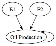
The conservative forecast above essentially takes both the E1 and E2 errors into account when computing prediction intervals for oil production since E1 is transmitted indirectly through the WL20 state variables.

A question at this point would be what if we ignored the E1 path entirely and just predict Oil Production without any input variables, what I would call a business as usual or BAU forecast. The Hubbert curve or Hubbert peak models were essentially BAU models with a different functional form i.e., the Logistic Distribution Curve. The advantage of the BAU models is that there is no cascading uncertainty. The BAU forecast in the graph above predicts that oil production will approach a peak somewhere between 80 million and 140 million tons of oil equivalent and stay there forever. This forecast is probably consistent with the improbable upper prediction interval of our initial conservative forecast.

Aside from the fact that we know oil is a nonrenewable resource, why should we prefer any of these plausible forecasts over any of the others? If we limit ourselves to the step-ahead AIC criteria, the BAU model is the winner with [264.70 < AIC=240.18 < 309.53] compared to the world system model with [290.42< AIC=279.72 <315.11]. However, if instead we calculate the attractor-based AIC, the WL20 model is best with AIC = 278.58 as compared to AIC=538.30 for the random walk model and AIC=315.06 for the BAU model. In other words, the BAU model is good at predicting next year's oil production but not very good at looking 50 years into the future (recall that the attractor simulation starts in 1950 and, from that initial position, simulates oil production out to 2008).

My experience has been that single equation models such as the BAU model or the Logistic model, are good at step-ahead predictions and are not subject to cascading uncertainty from input variables. However, single-equation models are not necessarily very good at predicting into the future even if the confidence intervals look quite narrow. And, because attractor models describe a path the system wants to move toward, their predictions also make more theoretical sense. The key here is to run the attractor simulation and compare the AICs for that simulation rather than the step-ahead simulation.

The ultimate test of all this is to compare the actual path of oil production over the next thirty years to the predictions of the various models--I just won't be around to make that comparison. In the next post, I'll explain how to generate these forecasts for the next generation in case they are interested.

Peak Oil Forecast and Global Warming

Peak Oil is the point where the rate of petroleum extraction starts declining because the resource is being exhausted.  US domestic Peak Oil production was reached in 1970. World oil production may have peaked in 2011, but it is too early to establish that as fact. In this post, I will forecast World oil production using the WL20 model to see whether the model thinks the World system has reached Peak Oil.

If you've "peaked" at the graphic above you probably can determine that the answer will be "Yes"! However, there's much more at stake here than the simple conclusion, however controversial, that we have reached Peak Oil.

After seeing my Global Warming forecast (here), one of my readers wondered whether anyone had combined Peak Oil models and Global Warming models. He reasoned, correctly, that the  WL20 model was capable of exploring the link between Peak Oil and Global Warming. This post will explore that relationship.

The underlying theoretical model linking Peak Oil and Global Warming is pretty simple: (Oil Production) -> (CO2 Emissions) -> (Global Warming). You might disagree with this linear causal model, but assume for the moment that it is correct. Then, anything that reduces oil production, like Peak Oil, will reduce Global Warming. My Global Warming forecast (here) shows Global temperature peaking sometime between 2040 and 2060. My Peak Oil Forecast above shows that oil production has reached its peak and is likely to collapse entirely around 2040. The result would seem to confirm the simple theoretical model, but how are these two forecasts related within the WL20 model?

The WL20 model model is a state-space model with three state variables (these state variables were not imposed on the model a priori but were the result of the statistical analysis): the first state variable measures overall growth in the World system; the second state variable measures declining biodiversity; and, the third state variable measures increasing resource constraints in the commodity markets related to the Ecological Footprint. The three state variables are interrelated: increasing biodiversity is related to declining global temperature while  increased resource extraction through commodity markets and overall economic growth are related to positive increases in global temperature.

The early peak in oil production is just one of a number of negative feedback loops within the model. The negative feedback loops limit overall growth in the World system around 2040 (see the WL20 state-variable forecast here). Global temperature takes a few more decades to peak after that, but it is really the end of overall growth, not just Peak Oil, that eventually limits global temperature growth, at least in the WL20 model.

There seem to be very few studies that have pursued the link between Peak Oil and Global Warming possibly because there are many alternative, high-carbon sources of energy (tar sands and synfuel from coal being two examples) that could be substituted for oil. Others, such as Amory Lovins (here) have argued that "Efficiency is cheaper than fuel" and will, for economic reasons, eventually limit emissions along with cheaper green energy. The WL20 model is capable of making projections of economic efficiency, a topic I will have to return to in a future post. The difficulty with the "substitution" argument is the important extent to which the entire World system is built on the oil economy. Even though we switched from a coal- to an oil-based economy in the 20th Century, it's not clear that the next energy conversion will be that easy given the larger scale of the present World system.

`

The prediction of Peak Oil was initially made by M. King Hubbert, a Shell geoscientist who died in 1989. The Hubbert curve or Hubbert peak for the World system is displayed above (from this source). His forecast, based on logistic curve modeling, predicted that the peak in World oil production would occur in the year 2000. It serves as a warning that no forecasting model can really see into the future. The models are simply attempts to explore the future implications of the data and models available when the forecast was made.