What Happened to Labor's Share of National Income around 1970 and 2000?

This page is UNDER CONSTRUCTION.

Notes

The Neoclassical Causal Model

 

Why is the US Labor Share in Income Declining and Will It Stop?

This page is UNDER CONSTRUCTION. Your comments and answers to questions would be appreciated. The topic is by no means simple and easy to analyze!

Except for a peak in the year 2000 (graphic above), Labor's Share of national Income (Q/L) in the United States has been consistently declining. There are two outstanding questions: (1) Why? and (2) When will it stop or possibly reverse? This post tests seven State Space models of the US economy to decide which model best explains the decline and forecasts what might happen in the future under each of the different models. The "best" model explains the labor share time paths as a result of inputs from the World System in which the US Economy is embedded.

The competing explanations for the decline in Labor's share are:

• Technological Change Technology can be embedded in the Capital Stock and cheaper Capital can be Substituted for Labor.
• Dynamics of the US Economy Shocks to the economic system (for example, technological shocks) can lead, over time, to changes in Labor's Share.
• Globalization and the World System Labor income can be driven down by cheap global competition and rewards for capital-labor substitution (using the KOF Index of Globalization).

In the graphic at the start of this post, six of the models are compared against a Random Walk, that is, no explanation.

In Neoclassical Economic Theory, Labor's Share of National Income and Capitals's share are constant parameters. At equilibrium, both are constant. Over time, differences can result from shocks and resulting system dynamics.

In Marxist Theory, Labor's share is driven to the subsistence level necessary to reproduce labor. Profit is whatever is left over after subsistence wages are paid.

ChatGPT summarizes it's findings as:

Here is a Causal Diagram of the ChatGPT explanation.

or a Simplified Model:

From the AIC Statistics below, the WL20-Input Model is best. However, the BAU model is a close second and the confidence intervals overlap.

Notes

Questions

1. What policy measures (if any) would you recommend to address the decline in Labor's Share of National Income?
2. Develop the Causal Diagram above in Neoclassical From (see see this post).
3. Derive the Simplified model of Labor's share from the Causal Diagram above using Loop Reduction Rules.
4. In the references below, do you find the World System mentioned directly or just indirectly? Do you think this is an important omission?
5. Is it necessary to go on to test the structural models (Solow-Swan vs. Marx-Ricardo) to understand the decline in Labor'ss Share?

References

NY Times (Sep 7, 2026) Why is Labor's Share of National Income Declining Is Technology the most important factor?

BLS, Second Quarter 2026, Revised, Economic News Release Labor productivity by sector

IMF (2017) What Explains the Decline of the U.S. Labor Share of Income? An Analysis of State and Industry Level Data we find that in addition to changes in labor institutions, technological change and different forms of trade integration lowered the labor share. In particular, the fall was largest, on average, in industries that saw: a high initial intensity of “routinizable” occupations; steep declines in unionization; a high level of competition from imports; and a high intensity of foreign input usage.\

NBER (2018) Is Automation Labor-Displacing? Productivity Growth, Employment, and the Labor Share We find that automation displaces employment and reduces labor's share of value-added in the industries in which it originates (a direct effect).

BLS (2020) Assessing the Impact of New Technologies on the Labor Market: Key Constructs, Gaps, and Data Collection Strategies for the Bureau of Labor Statistics Private and public decisions related to labor markets and working conditions are increasingly being influenced by technological considerations. Spurred by a wave of technological developments related to digitization, artificial intelligence (AI), and automation, governments around the world have declared that the creation and deployment of these technologies present both important opportunities and challenges to their citizens.

AER (2022) The Decline of the Labor Share: New Empirical Evidence We use time series techniques to estimate the importance of four main explanations for the decline of the US labor income share: rising firm markups, falling bargaining power of workers, higher investment-specific technology growth, and more automated production processes ... Our results point to automation as the main driver of the labor share.

 

Wikipedia Links

• Solow-Swan  an economic model of long-run economic growth. It attempts to explain long-run economic growth by looking at capital accumulation, labor or population growth, and increases in productivity largely driven by technological progress. At its core, it is an aggregate production function, often specified to be of Cobb–Douglas type, which enables the model "to make contact with microeconomics".
• Marxian Economics  a heterodox school of political economic thought. Its foundations can be traced back to Karl Marx's critique of political economy.
• Ricardo: Iron Law of Wages a proposed law of economics that asserts that real wages always tend, in the long run, toward the minimum wage necessary to sustain the life of the worker. The theory was first named by Ferdinand Lassalle in the mid-nineteenth century. Karl Marx and Friedrich Engels attribute the doctrine to Lassalle (notably in Marx's 1875 Critique of the Gotha Program), the idea to Thomas Malthus's (1798) An Essay on the Principle of Population, and the terminology to Goethe's "great, eternal iron laws" in Das Göttliche.
• Akaike Information Criterion (AIC) an estimator of prediction error and thereby relative quality of statistical models for a given set of data. Given a collection of models for the data, AIC estimates the quality of each model, relative to each of the other models. Thus, AIC provides a means for model selection.
• Labor's Share the wage share or labor share is the part of national income, or the income of a particular economic sector, allocated to wages (labor). It is related to the capital or profit share, the part of income going to capital, which is also known as the K–Y ratio. The labor share is a key indicator for the distribution of income.

Solow-Swan

In the Solow-Swan Neoclassical economic model, wages (W) and profits (R) have fixed parameters in the model, w and r respectively.

Marx-Ricardo

In the Marx-Ricardo model, the Iron Law of Wages determines that, in the long run, the wage parameter, (w), is fixed at the level of subsistence as a result of market pressure and capitalist exploitation.

AIC Statistics

In terms of the AIC Statistics (smaller is better), the best model takes the World System (WL20 model) as input.

TECHE Forecast: Union Membership

Union Membership is forecast to be zero around 2060 as a result of Technical Efficiency Changes (TECHE). However,

There is not a lot of separation between the model AIC Statistics (above) and their confidence intervals.

TECHE Forecast: KOF Globalization

The KOF Index of Globalization is forecast to continue growing beyond 2100.

USL201 Forecast: W Index

The WL20 Model is in growth-and-collapse mode and is forecast to peak after 2050.

 

World-System (1970-2100) World Population Collapse

October 27, 2025. NPR ran a segment on how Populations are Shrinking and Altering the Global Economy. It is somewhat surprising that Population Decline has not been bigger news. It has been going on in many countries and for the entire World System (graphic above with 98% bootstrap prediction intervals).

The United Nations has essentially been making Population projections (graphic above) similar to my WL20 Model at the start of this post.

The basic theoretical model underlying the possible impact of Population Decline is the Kaya Identity (above) used by the IPCC to help understand Global Temperature Change. The Kaya Identity is true by definition (see the Boiler Plate) so any decrease in Population will not only decrease economic growth (Q) but also decrease CO2 emissions and moderate Global Temperature (T).

My models are also predicting that growth in the World System will peak before 2100 (here) as will Global Temperature (here). The reasons are that there are powerful negative feedback loops from environmental and market controllers that eventually limit growth of the World System. 

Exercises

You can experiment yourself with one of my World System models here. The models are written in the R programming language and can be run on line. Suggestions in the code, to include bootstrap confidence intervals for choosing reasonable counterfactuals, can be found in the code. The model is stable and cyclical.

Another one of my World Systems models is unstable and produces exponential growth forever (here). When it is stabilized (instructions in the code) the World System reaches a steady state after 2100.

The future could be any one of these models or something else entirely (see the Boiler Plate for IPCC Emission Scenarios). You have to ask yourself which one of the models (if any) seem reasonable.

Can every country have the US standard of living?

The field of Development Economics is based on the idea of Convergence: Because underdeveloped economies have faster growth rates than developed economies, all economies will eventually converge in terms of per capita income (taken as a proxy for the standard of living). Convergence holds out hope to developing economies: adopt Western economic models, open your economies to global trade and eventually your citizens will enjoy the same high standard of living as the US. 

Unfortunately, the Convergence model is based on three faulty assumptions: (1) Every economy has basically the same underlying economic model differing only in parameter values, (2) We only need to consider economic variables e.g., Gross Domestic Product (GDP) and (3) There is no such thing as a world-system, we only have isolated countries that can interact independently through global trade.

The first two assumptions can be summarized with the Neoclassical Economic Growth Model (the Solow-Swan Model with a Cobb-Douglas production function).

The causal directed graph (path diagram) for the model is displayed above. One portion of the population (N) is employed as labor (L). Labor and exogenous technological change (T) drive output (Q). Capital stock (K) and Energy Consumption (E) are endogenous variables, that is, produced through economic activity. The final output is Consumption (C).  If the model is estimated from data, there can also be error terms and shocks (V2 and V3). Sometimes land (NR, natural resources) is included as an input, but often resources are ignored.

Every country is assumed to have the same basic economic models (see for example the William Nordhaus DICE and RICE models) differing only in parameter values (rates of population growth, rates of technological change, labor productivity, rates of investment, etc.). If you accept the model, it is easy to reason that rapid population growth and rapid technological change will lead to higher capital investment, higher consumption (but not necessarily consumption per capita) and higher energy use. Since there is typically higher population growth in less developed economies and since technology (knowledge) is a public good, then the predicted catch-up or convergence follows directly from the model. Needless to say, not all economists agree with the model or agree that it is supported by data, but enough do so that it contains the dominant thinking on economic growth. 

The model is myopic; it ends with consumption and energy use but does not consider the environmental impacts. The assumed counterfactual is that all countries can reach the US standard of living without environmental impacts. We can include a measure of environmental impact by adding the Ecological Footprint (EF) to the model (but see the WARNING note below). The EF measures the human demand on nature. It compares human consumption of environmental resources (demand) to biological capacity (BioCap in the directed graph above, environmental supply). Biocapacity is the biologically productive area within the country, a measure that is different from total land area because some land is unproductive (e.g, the majority of land underneath major metropolitan areas or in deserts). The ratio of consumption per capita to biocapacity per capita measures the EF or carrying capacity of the physical environment. If consumption exceeds biocapacity, the level of consumption is not sustainable unless supplemented by trade or unless technological change increase biocapacity. Obviously, not all countries can exceed biocapacity and make it up through trade. Carrying capacity without trade can be exceeded in the short run but is eventually unsustainable because the environment continues to loose biocapacity (the self-loop in the directed graph), that is, looses the ability to meet the demands placed on it.

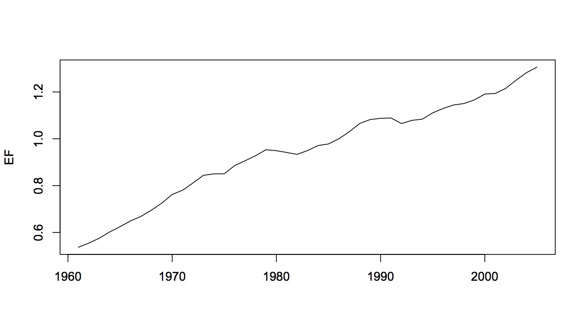
The EF for the world system is displayed in the first time series plot at the start of this post. Somewhere around the 1990s, the world system supposedly exceed it's carrying capacity (EF > 1.0). The world system did not collapse in the 1990s but, by this measure, we have been degrading our environmental support systems since then.

We can run some simple counterfactuals with EF data. For example, the graph above assigns US consumption levels to every individual in the world population but assumes no improvement of biocapacity. By 2020 (forecasting using the WL20 model), we would need the current biocapacity of almost five Earths to meet consumption demand.

If we were to assume that biocapacity of the entire world system reached the current biocapacity of the US, we would top out at around 2.5 Earths by 2500. It seems unlikely that biocapacity will reach US levels throughout the world, especially in arid countries. A reasonable prediction might be somewhere between these two forecasts.

The conclusion from this exercise is that convergence between all the economies in the world-system is seems unlikely. The US lifestyle is, in this sense, unsustainable. Either the US (and a few other Northern countries) will have to reduce its standard of living, be forced to reduce its standard of living (the ecological collapse after 2050 in the first forecast) or it will always have dominant economies. Even if the US would gladly reduce its standard of living to some low level (it's unlikely that any economy would) what would that level be and how many people in the world system could share it without degrading environmental systems? And, what will happen when the less developed world realizes that there is no hope of sharing Western standards of living? And, what might the world look like after an ecological collapse? More importantly, since the future really cannot be known, what do less developed countries do in the short run? I'll address that question in future posts.

WARNING: The Ecological Footprint (EF) is a measure which has been widely criticized and, at one extreme, called scientifically useless. From a statistical perspective, these critiques describe construct validity: does the EF construct measure what it claims to measure. There are many arbitrary assumptions in the construction of the EF (that is, the one supplied by the Global Footprint Network and used above) and the EF has become overburdened with sustainability interpretations that make it hard to know what is "supposed" to be measured. But there are other types of validity: face validity (does the measure superficially look right), content validity (are the right indicators being included in the measure) and criterion validity (is the measure useful in models and is it related to other measures in a reasonable way). My interest has been in the criterion validity of the EF. As can be seen above, it is useful in models and can be predicted (the dashed blue and green lines are the 98% bootstrap prediction intervals). Does it really mean that we might use five times our current biocapacity at some time in the future? No! If we give up the idea that this must be an absolutely correct measure, we can still ask relative questions that are interesting: how does it change over time and in different countries? How is it related to other measures of economic development? Can we construct alternative EF measures and how do they correlate to the one provided by the Global Footprint Network. I'll present some of this analysis in future posts.

US Retail Sales

Retail sales became the object of controversy this year when Paul Dales of Capital Economics challenged the "conventional wisdom" that Black Friday sales are a good predictor of yearly sales. In other places (here and here) I've described how the methodology used by Mr. Dales is probably flawed (I actually don't know what methodology was used but I made some guesses based on computer simulation). Another questionable part of Mr. Dale's work is the idea that any week during the year would be a good predictor of yearly sales. Sales forecasts would typically be based on some type of macro-economic time series model that uses multiyear data, the more the better. In this post, I will use multiple state space models to predict US retail sales. The results suggest a different story about what drives yearly sales in the US retail sector.

The Financial Forecast Center generates forecasts of US Retail Sales Growth Rates (here). The current forecast is displayed in the graphic above. The forecasts are generated with artificial intelligence software, not macro-economic models. As such, the FFC models do not have the biases associated with models based on a priori theoretical considerations. Their results show that retail sales growth rates have been declining since 2010 and are predicted to drop below 2% by 2013.

The FFC provides monthly, not seasonally adjusted, retail sales data (RSAFSNA) taken from the US Department of Commerce (here) in millions of dollars starting in 1992. When we plot that data for the period 2007-2012 (from the beginning of the financial crisis to the beginning of this year) we see very clearly that retail sales are elevated during the last two months of each year and that peak year-end sales pretty much follow trends for the rest of the year. The graph alone refutes the idea that Black Friday is a bunch of meaningless hype.

All this still begs the question of what is the best predictor of US retail sales. My approach is different from other forecasts that rely on models. Rather than advancing one model based on some argument, I test multiple models and choose the best one based on the AIC criterion: the best model is the one that predicts the historical data best with the fewest parameters. In this case, I tested the following models: (1) a random walk, R(t) = R(t-1) + E where R is Retail Sales and E is error, (2) a business-as-usual model, R(t) = a R(t-1) + E, (3) a state space model of the US economy, R(t) = a R(t-1) + S(US) + E where S(US) is the state of the US economy and (4) a state space model of the world economy,  R(t) = a R(t-1) + S(W) + E where S(W) is the state of the World economy. The states of the US and World economy are generated by the USL20 and WL20 models, respectively.

The rationale for these models is pretty straight forward: (1) given the high variability of the data, next year's sales may well be dominated by random error (the random walk), (2) if we smooth out some of the seasonal variability, average sales might just be a little bigger this year than last year (business-as-usual), (3) more realistically, US retail sales might depend on the entire state of the US economy and (4) given the globalization of world trade in retail services, the state of the world economy may be a better predictor of US sales.

The winner of the AIC competition was in fact the World economy model. The forecast with 98% prediction intervals from 2007-2015 is presented above. The best performance for retail sales was in 2007 and 2008. The worst performance was in 2009 and the first months of 2010. The sector has now pretty much recovered along with growth in the World economy. Returning to the FFC forecast of US retail sales growth rates, the forecast predicts an average annualized yearly growth rate of 2.07% for the period 2012-2015, very close to the current FFC number.

We've come a long way from the idea that Black Friday Retail Sales might be considered a reasonable predictor for yearly retail sales and learned that the US Retail Sector is part of the World economy. We've also learned that end-of-year sales are improbably (outside the 98% prediction interval) important to the sector. And, we've learned that setting up a single model to test a false problem is not a particularly useful way to conduct research.

TECHNICAL NOTE: The RSAFSNA.model is available here. Instructions for using forecasting models are available here. Once you have the R program installed and the dse, matlab, and scatterplot3d packages installed, you can run the following commands from the R console to display how well the best RSAFSNA.model fits the data.

> W <- "Absolute path for location of ws procedures"

> setwd(W)

> source("LibraryLoad.R")

> load(file="WL20v3_model")

> load(file="ws_procedures")

> 

> W <- "Absolute path for RSAFSNA model"

> setwd(W)

> load(file="US_RSAFSNA_model")

> m <- getModel(RSAFSNA.model,type="world index")

> tfplot(m)

You will notice that the model does not track the month-to-month variability in RSAFSNA. If we wanted to better predict things like end-of-year sales bumps, we could use seasonal dummy variables coded for the months of interest, for example November and December.

If you are interested in how the other models did, enter

> tfplot(m1 <- getModel(RSAFSNA.model,type="rw"))

> tfplot(m2 <- getModel(RSAFSNA.model,type="us index")) 

> tfplot(m3 <- getModel(RSAFSNA.model,type="bau"))

The plots actually seem to do a little better job of tracking the month-to-month variability. However, the AIC still suggests that the world model is best, but not by a huge amount.

> z <- bestTSestModel(list(m,m1,m2,m3))

Criterion value for all models based on data starting in period:  10 

5301.765 5354.228 5318.493 5377.438 

If you want to see the entire forecast with 98% bootstrap confidence intervals, enter

> b <- getModel(RSAFSNA.model,type="boot forecast")

> tfplot(b,m)

Using Forecasting Models

In an earlier post (here) I explained how to use the WL20 model and the ws (world system) package. In this post, I will explain how to use forecasting models such as the one used to make my Peak Oil forecast (here).

Assuming that you have followed my earlier post, have R installed on your machine and have also installed the dse and the matlab packages successfully, the forecasting models are all available here. For this demonstration, download the PeakOilIndexModel to your working directory. Then you can enter the following commands at the > prompt in the R console:

> W <- "the complete path name for your working directory"

> setwd(W)

> source(file="LibraryLoad.R)

> load(file="WL20v3_model")

> load(file="ws_procedures")

> load(file="PeakOilIndexModel")

The available forecasting models can be seen by typing (a help file for all the ws package functions is available here):

> summary(OIL.model)

The resulting listing will show each of the available models. For example,

[1] "BAU"

Eigenvalues of system matrix

[1] 0.9836614

[1] TRUE

     Parameter     Mean Mean LCI Mean UCI P>=T[1] P< T[1]

[1,]  240.1784 288.4285 264.6985 309.5271       1       0

     Std. Dev.      Bias    Bias-z

[1,]  18.21428 -48.25009 -2.649025

attr(,"class")

[1] "boot"

[1] "STRUCTURAL"

NULL

The BAU (Business As Usual) entry shows a number of statistics used to evaluate the model. The Structural model displays NULL because no structural model was estimated.

The first statistic displayed for the BAU model is the eigenvalue of the system matrix. If all the eigenvalues are less than unity, the model is stable, which is displayed next as [1] TRUE. The next line shows the bootstrap distribution of the AIC statistic. The first value, 240.1784, is the sample AIC statistic. The second value is the bootstrap mean AIC statistic. The third and fourth values are the lower and upper 98% confidence intervals for the AIC statistic. The remaining values display probabilities, standard deviation and bias for the sample AIC statistic. If you want to inspect the BAU model, enter:

> getModel(OIL.model,type="bau")

Given the AIC statistics, the BAU model is the best one observed. For the forecast, however, I used the  best attractor model which you can display with

> getModel(OIL.model,type="best attractor")

The best attractor model is based on a free-simulation of each estimated model and is chosen using the AIC statistic from the free simulations vs. the actual data residuals. In this case, the world index model

> getModel(OIL.model,type="world index")

provides the best attractor simulation. You can get a flavor for the differences in the predictions from the two models by entering:

> tfplot(sim(getModel(OIL.model,type="bau")))

> tfplot(sim(getModel(OIL.model,type="world index"),sampleT=95,input=WL20.fx))

The BAU model predicts a gradual decline over time in the rate of oil production while the best attractor model shows a sharp peak-and-collapse between 2000 and 2020. 

Why should we be willing to choose one of these models over the other? One is best by conventional standards (step-ahead predictions using the AIC). Another is best by standards derived from attractor theory and application of the AIC criteria to the free simulations of each model. 

In future posts, I'll work through this issue and also reveal some more of the things you can do with the forecasting models using the dse and the ws packages. At this point, you should be able to at least load and inspect the models.

Peak Oil Forecast and Global Warming

Peak Oil is the point where the rate of petroleum extraction starts declining because the resource is being exhausted.  US domestic Peak Oil production was reached in 1970. World oil production may have peaked in 2011, but it is too early to establish that as fact. In this post, I will forecast World oil production using the WL20 model to see whether the model thinks the World system has reached Peak Oil.

If you've "peaked" at the graphic above you probably can determine that the answer will be "Yes"! However, there's much more at stake here than the simple conclusion, however controversial, that we have reached Peak Oil.

After seeing my Global Warming forecast (here), one of my readers wondered whether anyone had combined Peak Oil models and Global Warming models. He reasoned, correctly, that the  WL20 model was capable of exploring the link between Peak Oil and Global Warming. This post will explore that relationship.

The underlying theoretical model linking Peak Oil and Global Warming is pretty simple: (Oil Production) -> (CO2 Emissions) -> (Global Warming). You might disagree with this linear causal model, but assume for the moment that it is correct. Then, anything that reduces oil production, like Peak Oil, will reduce Global Warming. My Global Warming forecast (here) shows Global temperature peaking sometime between 2040 and 2060. My Peak Oil Forecast above shows that oil production has reached its peak and is likely to collapse entirely around 2040. The result would seem to confirm the simple theoretical model, but how are these two forecasts related within the WL20 model?

The WL20 model model is a state-space model with three state variables (these state variables were not imposed on the model a priori but were the result of the statistical analysis): the first state variable measures overall growth in the World system; the second state variable measures declining biodiversity; and, the third state variable measures increasing resource constraints in the commodity markets related to the Ecological Footprint. The three state variables are interrelated: increasing biodiversity is related to declining global temperature while  increased resource extraction through commodity markets and overall economic growth are related to positive increases in global temperature.

The early peak in oil production is just one of a number of negative feedback loops within the model. The negative feedback loops limit overall growth in the World system around 2040 (see the WL20 state-variable forecast here). Global temperature takes a few more decades to peak after that, but it is really the end of overall growth, not just Peak Oil, that eventually limits global temperature growth, at least in the WL20 model.

There seem to be very few studies that have pursued the link between Peak Oil and Global Warming possibly because there are many alternative, high-carbon sources of energy (tar sands and synfuel from coal being two examples) that could be substituted for oil. Others, such as Amory Lovins (here) have argued that "Efficiency is cheaper than fuel" and will, for economic reasons, eventually limit emissions along with cheaper green energy. The WL20 model is capable of making projections of economic efficiency, a topic I will have to return to in a future post. The difficulty with the "substitution" argument is the important extent to which the entire World system is built on the oil economy. Even though we switched from a coal- to an oil-based economy in the 20th Century, it's not clear that the next energy conversion will be that easy given the larger scale of the present World system.

`

The prediction of Peak Oil was initially made by M. King Hubbert, a Shell geoscientist who died in 1989. The Hubbert curve or Hubbert peak for the World system is displayed above (from this source). His forecast, based on logistic curve modeling, predicted that the peak in World oil production would occur in the year 2000. It serves as a warning that no forecasting model can really see into the future. The models are simply attempts to explore the future implications of the data and models available when the forecast was made.