US Inflation by Administration

 

We are now within a week of the 2024 Presidential Election. There seems to be a lot of confusion in the American electorate about the state of the Economy and the role (if any) that has been played by prior administrations. In a earlier post (here), I looked at GDP across eight Administrations starting in 1974 (I also explain how to read the graphic above). In this post, I will look at Inflation, specifically the Consumer Price Index (CPI).

There were two major episodes of Inflation since 1974:  (1) The Great Inflation of the late-1970s and early 1980s and (2) the COVID-19 Pandemic Inflation of 2020. Both these historical periods provide fascinating Economic History and provide clues about how the Economic System really works (particularly the Nixon Price Controls and the current debate). Commentators with an axe to grind will argue that inflation is caused by Government Expenditure. For example, the Inflation Reduction Act of 2022 is erroneously argued to have caused the Inflation of 2020, but causation doesn't run backwards in time. 

Without becoming sidetracked in the causes of Inflation (I'll address that elsewhere), the major causes of Inflation in the Modern period are economic Shocks (the first row of the figure above):  

Since 1975, we've had (1) the Vietnam War, (2) the Great Society Programs, (3) the Arab Oil Embargo, and (4) the COVID-19 Pandemic. Everyone reading this lived through the COVID-19 Pandemic and experienced  supply chain disruptions (remember hoarding toilet paper). Any supply shocks will increase prices--that's simple ECON 101. Aggregate Demand shocks can also increase inflation, but the effects pale by comparison. 

It's inevitable that the current administration (Carter in the late-1970s and Trump in 2020) gets blamed for everything that happens on their watch. Except for botched or nonexistent attempt at Price Controls (they were used effectively during WWII), the shocks that hit the Economic System and resulted in Inflation had external causes. It is really the Political System's response or poor memory of cause-and-effect that has led to a bad taste in Voter's mouths.

In any event, the COVID-19 Pandemic Inflation is over, the  Inflation Reduction Act of 2022 has not created permanent increases in the CPI and the Atlanta Fed Economy Now App (you can get it on your cell phone and the forecasting approach is similar to the one I use) also predicts declining Inflation.

My take on the current Inflation episode is that the Political System missed an opportunity to implement a reasonable, possibly temporary, regime of Price Controls. For example, the Kroger-Albertson's Supermarket Merger  which was blocked by the Federal Trade Commission (FTC) could have been used to exert some control over Food Prices. As a condition of the merger, the new company would have been required to accept Price Gouging laws. Food Price Inflation has been major complaint of consumers. Capping price increases at Kroger-Albertson's would have been a major stimulus to their business. Blindly following Neoliberal Free-Market principles has prevented the US from responding to Inflation. Voters should be concerned about failures in the Political System.

US Economic Performance by Administration

 

We are about a week away from the US 2024 Presidential Election. Polling seems to show that likely voters are very concerned about the economy and hold each succeeding administration responsible for economic performance (see below). 

The graphic above shows Gross Domestic Product (GDP) performance since 1975 by the various presidential administration. The black line is actual GDP, the dashed red line is the GDP Attractor Path and the dotted and dashed blue and green lines are the lower- and upper-98% prediction intervals, respectively. The model used for prediction is my version of the Atlanta Fed GDP Now model.

The model shows that for most of the period (except briefly in the Reagan administration) the economy performed better than might have been expected from the Attractor Path. The Clinton and Bush II administrations even briefly reached the upper-98% prediction interval. The Trump administration inherited a solid economy from the Obama administration but was clearly affected by the COVID Pandemic. The Biden administration, so far, has almost returned to the upper-98% prediction interval, meaning the economy has performed extraordinarily well.

The best prediction for the future is that the economy will return to the GDP Attractor Path which means that whichever party wins the White House, the administration will face downward pressures on economy growth.

Polling on Economic Performance

A recent CBS poll (here) shows that respondents rated the prior Trump Administration (Jan 2017 to Jan 2021) as better than the current Biden Administration on economic performance. The polling does not seem to reflect the actual data (see above) but the COVID Pandemic hit during the Trump administration and respondents seem to discount the resulting economic shocks.

Update

Current BEA estimates (here) show GDP increasing within the upper-98% prediction interval. The economy continues to perform quite well inspite of pessimistic polling data.

Was It a Mistake for Britain to Enter the EU?

I have written an earlier post (here) showing the effect on Gross Domestic Product (GDP) of Britain leaving the EU and pursuing a Go-It-Alone Scenario. The effect, based on the UK20 model run with no inputs, was that GDP would peak in 2020. The pro-BRitain EXIT (Brexit) model makes the argument that Britain should have never joined the EU. I will investigate that counterfactual in the following post.

The way to construct a BrNoEU (Britain No EU) counterfactual would be to estimated a statistical model using only data prior to the assumed entry point. Then the model prediction for some variable, such as GDP, would be forecast into the future and compared with what actually happened. If entering the EU was good for GDP, the fictitious future should have shown slower growth than actually happened.

The history of Britain's entry into the European Union (EU) is somewhat complex (here), but let's for the sake of simplicity use the signing of the Maastricht Treaty on Nov 1, 1993 as the starting point. For a number of reasons to be discussed next, I decided to start the model in the year 2000 and do an attractor-path simulation with the UK2000 model model starting in 1960. The best UK2000 model has no inputs meaning that the best way to think about Britain in the late 20th century was as a Go-It-Alone nation.

To understand the counterfactual, look at the time plot above. The dark solid line is the actual path of GDP displayed here from 1980 to 2012. The dashed red line is the attractor path constructed by simulating the UK2000 model from 1960 to 2040. The dashed green and blues lines are the 98% upper and lower prediction intervals. The prediction intervals are relatively narrow for the period where we have data and start to get wider apart in the future as our confidence in the prediction decreases.

Looking at the actual path for GDP (dark solid line), prior to the Maastricht Treaty, Britain was having some trouble staying on the attractor path. The economic bubble that started in the mid-1980s had popped by the point the Maastricht treaty was signed. At the time, it must have looked as if Britain needed some help maintaining economic growth and joining the EU offered that hope. Indeed, from the 1990s till the Financial Crisis of 2007-2008, it looked as if joining the EU had been a success. The hope that Britain would keep growing (red arrow) above the attractor path, however, was an unrealistic expectation. Currently, the British economy is on the attractor path looking as if there was not much benefit from entering the EU.

How do we understand this counterfactual? If the pro-Brexit position is that the British economy would return to the growth rates of the 1993-2007 period by leaving the EU, the model shows that joining the EU would most likely lead to the departure from the attractor path and the 2007-2008 Financial Crisis put an end to the boom. The pro-Brexit position confuses membership in the EU with the effects of the 2007-2008 Financial Crisis. Leaving the EU will not increase GDP growth and will likely take the British economy back to the boom-and-bust period of the 1980s.

If you look back at my earlier post (here), you will also see that whatever Britain does, attractor path growth for the economy is slowing. The economy is maturing and Brexit will not change that and will probably only make matters worse. This, of course, would not be an easy argument to sell to the British public.

Can every country have the US standard of living?

The field of Development Economics is based on the idea of Convergence: Because underdeveloped economies have faster growth rates than developed economies, all economies will eventually converge in terms of per capita income (taken as a proxy for the standard of living). Convergence holds out hope to developing economies: adopt Western economic models, open your economies to global trade and eventually your citizens will enjoy the same high standard of living as the US. 

Unfortunately, the Convergence model is based on three faulty assumptions: (1) Every economy has basically the same underlying economic model differing only in parameter values, (2) We only need to consider economic variables e.g., Gross Domestic Product (GDP) and (3) There is no such thing as a world-system, we only have isolated countries that can interact independently through global trade.

The first two assumptions can be summarized with the Neoclassical Economic Growth Model (the Solow-Swan Model with a Cobb-Douglas production function).

The causal directed graph (path diagram) for the model is displayed above. One portion of the population (N) is employed as labor (L). Labor and exogenous technological change (T) drive output (Q). Capital stock (K) and Energy Consumption (E) are endogenous variables, that is, produced through economic activity. The final output is Consumption (C).  If the model is estimated from data, there can also be error terms and shocks (V2 and V3). Sometimes land (NR, natural resources) is included as an input, but often resources are ignored.

Every country is assumed to have the same basic economic models (see for example the William Nordhaus DICE and RICE models) differing only in parameter values (rates of population growth, rates of technological change, labor productivity, rates of investment, etc.). If you accept the model, it is easy to reason that rapid population growth and rapid technological change will lead to higher capital investment, higher consumption (but not necessarily consumption per capita) and higher energy use. Since there is typically higher population growth in less developed economies and since technology (knowledge) is a public good, then the predicted catch-up or convergence follows directly from the model. Needless to say, not all economists agree with the model or agree that it is supported by data, but enough do so that it contains the dominant thinking on economic growth. 

The model is myopic; it ends with consumption and energy use but does not consider the environmental impacts. The assumed counterfactual is that all countries can reach the US standard of living without environmental impacts. We can include a measure of environmental impact by adding the Ecological Footprint (EF) to the model (but see the WARNING note below). The EF measures the human demand on nature. It compares human consumption of environmental resources (demand) to biological capacity (BioCap in the directed graph above, environmental supply). Biocapacity is the biologically productive area within the country, a measure that is different from total land area because some land is unproductive (e.g, the majority of land underneath major metropolitan areas or in deserts). The ratio of consumption per capita to biocapacity per capita measures the EF or carrying capacity of the physical environment. If consumption exceeds biocapacity, the level of consumption is not sustainable unless supplemented by trade or unless technological change increase biocapacity. Obviously, not all countries can exceed biocapacity and make it up through trade. Carrying capacity without trade can be exceeded in the short run but is eventually unsustainable because the environment continues to loose biocapacity (the self-loop in the directed graph), that is, looses the ability to meet the demands placed on it.

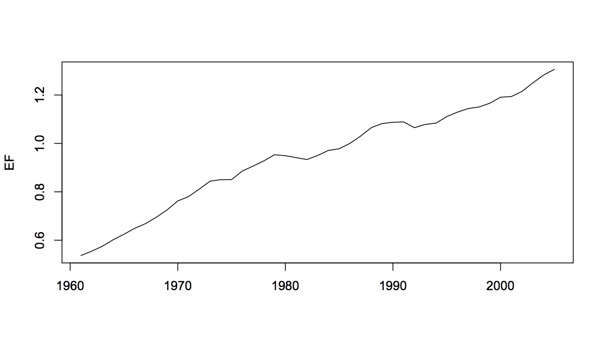
The EF for the world system is displayed in the first time series plot at the start of this post. Somewhere around the 1990s, the world system supposedly exceed it's carrying capacity (EF > 1.0). The world system did not collapse in the 1990s but, by this measure, we have been degrading our environmental support systems since then.

We can run some simple counterfactuals with EF data. For example, the graph above assigns US consumption levels to every individual in the world population but assumes no improvement of biocapacity. By 2020 (forecasting using the WL20 model), we would need the current biocapacity of almost five Earths to meet consumption demand.

If we were to assume that biocapacity of the entire world system reached the current biocapacity of the US, we would top out at around 2.5 Earths by 2500. It seems unlikely that biocapacity will reach US levels throughout the world, especially in arid countries. A reasonable prediction might be somewhere between these two forecasts.

The conclusion from this exercise is that convergence between all the economies in the world-system is seems unlikely. The US lifestyle is, in this sense, unsustainable. Either the US (and a few other Northern countries) will have to reduce its standard of living, be forced to reduce its standard of living (the ecological collapse after 2050 in the first forecast) or it will always have dominant economies. Even if the US would gladly reduce its standard of living to some low level (it's unlikely that any economy would) what would that level be and how many people in the world system could share it without degrading environmental systems? And, what will happen when the less developed world realizes that there is no hope of sharing Western standards of living? And, what might the world look like after an ecological collapse? More importantly, since the future really cannot be known, what do less developed countries do in the short run? I'll address that question in future posts.

WARNING: The Ecological Footprint (EF) is a measure which has been widely criticized and, at one extreme, called scientifically useless. From a statistical perspective, these critiques describe construct validity: does the EF construct measure what it claims to measure. There are many arbitrary assumptions in the construction of the EF (that is, the one supplied by the Global Footprint Network and used above) and the EF has become overburdened with sustainability interpretations that make it hard to know what is "supposed" to be measured. But there are other types of validity: face validity (does the measure superficially look right), content validity (are the right indicators being included in the measure) and criterion validity (is the measure useful in models and is it related to other measures in a reasonable way). My interest has been in the criterion validity of the EF. As can be seen above, it is useful in models and can be predicted (the dashed blue and green lines are the 98% bootstrap prediction intervals). Does it really mean that we might use five times our current biocapacity at some time in the future? No! If we give up the idea that this must be an absolutely correct measure, we can still ask relative questions that are interesting: how does it change over time and in different countries? How is it related to other measures of economic development? Can we construct alternative EF measures and how do they correlate to the one provided by the Global Footprint Network. I'll present some of this analysis in future posts.

No, Q3-2017 3% GDP growth does not support Big Tax Cuts!

The Washington Post recently published an article titled Third quarter's strong economic growth could boost GOP tax effort. The article predicts the Trump administration will make the case that if you want economic growth to keep increasing to 4% (President Trump's goal), we need tax cuts. The Financial Forecast Center (here) predicts GDP Growth Rates out to the end of 2017 (graphic above). The forecast graph does not even have room for 3%, let alone 4%, GDP growth this year. Who is right?

The GOP tax cut plan is based on a long chain of reasoning. Tax cuts are supposed to increase investment and consumption (I = iY - T and C = cY - T). Investment and consumption are supposed to increase National income (as does Government expenditure and the Balance of Payments, Y = I + C + G + BOP). On the other hand, tax cuts increase the deficit D = G - T which is supposed to crowd out investment through the interest rate effect (increased interest rates discourage borrowing). Any one of these effects could fail to materialized or provide only a short term boost to the economy when the Deficit chickens come home to roost.

Let's ask a more systemic question: What kind of growth rate is the US economy capable of sustaining? Another way to state the question is to ask what is the attractor path for GDP growth? The  attractor path for the annualized growth of US GDP (based on quarterly data, here) is displayed above. Out to 2030, the attractor path (the dashed red line based on the state of the US economy from the USL20 model*) is stable at around 2%. The 98% bootstrap prediction intervals (the dashed green and blue lines) suggest that numbers from 1.5% to 2.5% are probable. Growth rates above 3.5% or even negative are possible but the economy will return over time to around 2%. This is the growth rate that the US Economy can reasonably sustain given the current physical structure and economic organization. 

The real growth of the US economy, Q = f(K,L,Tech), is based on how capital, labor and technology are combined. Changes in who has money may or may not make a difference to the physical structure and economic organization of the US economy. The excess money available from tax cuts (especially if directed at the wealthy) can be spent on luxury goods or stock market speculation, neither of which will build economic capacity through investment and employment. 

If the fractured GOP is able to legislate tax cuts, time will tell how the US economy is affected. The most likely prediction is that high growth rates, if they happen at all, would be very temporary.

_____

* The best model (determined by the AIC criterion) is ag(GDPQ)(t) =  (F)ag(GDPQ)(t-1) + G(S)(t-1) + Qe(t), where ag() is annualized growth, F, G and Q are coefficient matrices, S is the state vector from the USL20 model and e(t) is random error. The current upsurge in US GDPQ is driven by e(t).

Coal Will Make Reducing Energy Intensity Difficult

May 26, 2026 Scientist Ditch Scary Climate Scenario Goodbye RCP8.5 (see below). A Problem with RCP8.5 was the overly pessimistic projection for coal use and it's environmental impact.

The New York Times ran an article on Aug 30 titled The Challenge of Cutting Coal Dependence. The article focuses on the problems Germany, "a leader in the push against climate change", is having reducing dependence on coal production. Coal is Germany's main and dirtiest source of electricity generation. And, the same is true for many other countries, for example the US, China, and India. The problem is how to replace all the jobs that would be lost. No one has a practical answer. 

The graph above of coal consumption over time (from the NYT article) shows that Germany and the US have basically stabilized their coal consumption. The rest of the World, on the other hand, has not. My main question, when I read the article, was what can we expect from the future.

The graph at the beginning of this post is a forecast of coal production based on the WL20 model (the forecast assumes no policy intervention in the future). It shows that, with relatively narrow bootstrap 98% prediction intervals, coal production will not stabilize until well after the year 2100.

Compare that forecast to the one, also drawn from the WL20 model, of oil production. The model predicts that oil production has peaked, again with a high degree of confidence, and will decline for the foreseeable future (with or without policy intervention).

While commentators have been optimistic about the role reduced oil production will have in future carbon emissions, they have missed the major roadblock to reducing carbon intensity. Coal is a plentiful and easily obtained resource. Mining coal creates jobs. The NY Times article concludes with a quote from Craig Morris, an environmental blogger: "Several degrees of warming by 2100 may sound scary, but not nearly as much as long-term joblessness just a few years from now."

Notes

My Global Temperature Projections aren't as bad as RCP8.5 or other worst-case scenarios. The reason is that World System Collapse reduces the drivers of climate change in World System input models.

For more information about data sources and how the State Space models were constructed, see the Boiler Plate.

Carbon Brief (21 August 2019) Explainer: The high-emissions 'RCP8.5' global warming scenario.

WL20 Measurement Model

The measurement model for the World System has three historical environmental controllers: W1=(Growth-LivingPlanet), W2=(LivingPlanet-TEMP) and W3=(P.Oil.-TotalFootprint).  Information about the indicators (LivingPlanet index, Global TEMP, TotalFootprint), etc. can be found in the Boiler Plate.

** Recent data from NASA's CRES (Clouds and Earth’s Radiant Energy System) satellite data also indicates that Earth's Albedo (ability to reflect sunlight and reduce warming) is decreasing!

RCP Projections

RCP2.6 to RCP8.5

Although there has been a lot of controversy surrounding RCP8.5 (Scientist Ditch Scary Climate Scenario), one point to make about the graphic above is that there is no Unlimited-Exponential-Growth-Forever scenario which seems to be what Climate Deniers predict will happen. Neoclassical Economists (see the DICE model) argue that growth will be limited when Technological change (Productivity) and Population growth reach a steady state (See the Solow-Swan Neoclassical Growth Model below).

Solow-Swan Growth Model

The Solow-Swan Neoclassical Growth Model (the basis for the DICE model) is one of the most important macro models in economics (along with the AS-AD Supply-Demand model). The directed graph above shows that the two exogenous causal variables are Population (N) and Technology (TECH). If either of these variables stop growing, the system will reach a Steady State Economy. It may be surprising to students of Economics to learn that, from a causality standpoint, Labor (L), Production (Q) and Capital Stock (K) are dependent variables and are not the primary drivers of growth in the  Solow-Swan Neoclassical Growth Model.

UN Population projections currently anticipate that Population will peak at 10.3 Billion people in 2084. In order to reach a Steady State Economy, the  DICE model has to also assume (arguably) that Technology Change will also peak at some time in the future.

Should Britain Exit the EU (Brexit?)

The PBS News Hour featured a segment tonight (above and here) asking whether "...the economic cost of Brexit is too great?" Brexit stands for BRitain EXiting the European Union. The United Kingdom European Union Membership Referendum will be held on June 23, 2016 to decide the issue.

In the video above, the News Hour presented an interesting debate held at the Oxford Union where heavy weight politicians made the case for and against Brexit. The arguments are interesting and well stated but seemed to be based on the idea that "since no one can know what will really happen," the issue must be resolved by debate. In the end, most of the students attending voted to stay in the EU.

The reason "no one can know the outcome" is that Brexit involves a counterfactual. No country has ever exited the EU and there is no historical experience that can be applied to decide what might happen if Britain did. As readers who follow Fact, Fiction and Forecast know, historical data can be applied to the question if you have models of both the British and the EU economies and if those models can be simulated under different conditions. The challenge is to choose those "different conditions" in a convincing manner.

Without going into a great deal of detail, two state models are available: UK20 and EU20. For the late 20th and early 21st century, the EU20 model is primarily being driven by the world system (outputs for the WL20 model) while the UK20 model is primarily being drive by outputs from the EU20 model. One might easily jump to the conclusion that since the UK20 model was primarily driven by the EU20 model, the logic of staying in the EU is obvious. However, the real counterfactual question is what will happen in the future.

To pose this question, I simulated the UK20 model being driven by the EU20 model and then simulated a version of the UK model with no inputs (the Go-it-Alone scenario). If the EU has been holding back the UK, this comparison would demonstrate the drag being placed on the UK by EU membership. Go-it-Alone is not the only possible strategy for the UK (I'll talk about that below) but these two models are actually the best models for the UK economic system when compared against a number of other competitors.

The graphic above is the attractor path simulation of UK GDP using the state of the EU20 model as input. The red dashed line is the attractor path. The green and red dashed lines are the 98% bootstrap prediction intervals. With a high degree of confidence, the model predicts that the British economy will peak sometime in the 2030s.

The next graphic above is a free simulation of the UK20 model starting in 1960 with no inputs (the Go-it-Alone scenario). In the alternate future, the EU economic system is predicted to peak in 2020 and decline rapidly after that. There is some probability that the economy might peak somewhat later in 2035 (the dashed green line), but there is a higher probability of significant decline after 2020. Also notice that the confidence intervals are wider meaning that this is a less precise prediction.

GDP isn't the only criterion measure we might look at (What about labor force issues? If you are interested, let me know). And, there are many other strategies Britain might choose after leaving the EU and Go-it-Alone is only one. Britain could choose to aline itself either with the US or with the entire World System, bypassing the EU. I have also estimated these alternative models and they are inferior to the ones presented above meaning that the prediction intervals would be even wider.

We will all have to wait for the referendum results on June 23, 2016 and then have to wait again for 2020, 2030, 2040 and 2050 to see what the future may hold. Myself and many of the "heavy weight politicians" who argued the case at the Oxford Union will no longer be alive to see the future that unfolds but many of the students will. Their intuitions, expressed in their votes, seems to favor staying in the EU (as does the counterfactual simulation, the fiction and the forecasts presented above).

EXTRA CREDIT

Assume that Britain stays in the EU.  There are people who now favor Brexit who will argue, at the first signs of slowing in the UK economy, that the reason is having chosen to stay in the EU. What will you say to them?