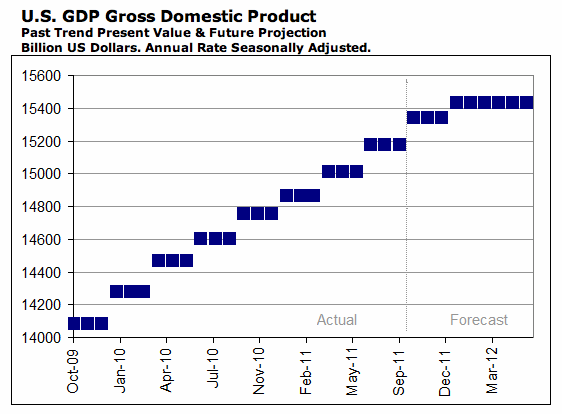
US Real GDP Growth in 2012

The Financial Forecast Center (FFC here) produces a forecast for US nominal GDP. From the graphic above, FFC is expecting little growth in the first two quarters of 2012. FFC presents two confidence bands for each value. For example, in Jan 2012, FFC is forecasting nominal GDP at $15,333B. The 50% correct band would be +/- 112 while the 80% correct band would be +/- 225. The bands get bigger over time as expected but the GDP value stays at $15,433B through June of 2012, the end of the FFC forecast period.
I would prefer to forecast real GDP since it would not be clear for a nominal GDP forecast how much trends would be affected simply by prices (the GDP deflator). I would also rather forecast the attractor value since we are just coming out of the Subprime Mortgage Bubble and Collapse.

My attractor forecast for real GDP taken from the BEA (here) is presented in the graphic above. The bubble and collapse is clearly displayed. Currently we are at the lower 98% prediction interval for the attractor. This suggests that GDP will be drawn higher in 2012 (a return to the attractor value) unless other events (such as the EU sovereign debt crisis) continue to weight down the US economy (the mechanism of transmission here could be either a reduction in US exports to the EU or more financial contagion).

The FFC does produce a US Real GDP growth rate forecast (here and in the graphic above). The FFC is predicting a reduction in real GDP growth down to around 0.6% in the second quarter on 2012 (50% +/- 1.1% and 80% correct +/-2.4%).

My average annualized growth rate forecast for 2012 is 1.5% which is close to the FFC forecast of 1.6% for the first quarter of 2012. The FFC forecast of 0.5% growth in the second quarter of 2012 is possible but not that likely since the economy is not on its attractor value in the first quarter of 2010.

As a comparison, my mean annualized attractor growth rate for the period 2004-2007 was 1.6% while the actual mean annualized growth rate was 2.5%, 1 full point being attributable to the bubble.

NOTE: The attractor value results from a free simulation of GDPC96 starting in 1960 being driven by the state variables from the WL20 model. The WL20 model produces the best attractor as determined by the AIC criterion. A typical forecast predicts from year to year. The prior year contains shock and bubble values that bias the forecast.

Canada Backs Out of Kyoto

On Monday, December 12, as an NPR Marketplace piece documents, Canada pulled out of the Kyoto Protocol blaming the lack of participation of the US and China in the accord. Under the Kyoto Protocol, Canada pledged to reduce its CO2 emissions by 6% compared to 1990 levels. In 2011, Canada decided to move the goal post and seek a 17% reduction from 2005 levels by 2020 (read the history here).

Unfortunately, Canada is nowhere close to meeting either of these goals and appears on a future path of increased emissions as long as I would feel comfortable forecasting into the future (attractor forecast above, dashed red line with 98% prediction intervals).

What's interesting is that Canadian CO2 emissions are being driven predominantly by the North American regional system, that is, by the combined productive power of the US and Canada. What is also interesting is that while US emissions have a chance of stabilizing by 2040 (see my forecast here), Canada's emissions do not.

The Canadian government is basically accurate in the reasons given for pulling out of Kyoto. If US energy demand (and thus CO2 emissions) is ever reduced, Canada will just continue exporting whatever hydrocarbons it can produce to China, India or whomever needs oil. The export orientation of Canada's economy is probably the reason that CO2 emissions are unlikely either to be reduced through international protocols or technological change.

US CO2 Emission Reductions Unlikely as a Result of COP17

COP17 (17th Conference of the Parties to the UNFCCC) started today in Durban, South Africa and a salient topic of discussion was what will happen when the Kyoto Protocol 2012 Emission Targets expire next year. Of particular concern is what the US will do. The graphic above is an attractor forecast out to 2050 for US CO2 emissions. It's useful to discuss the forecast in terms of the Kyoto Protocol.

The Kyoto Protocol was initially adopted in December of 1997, went into force in February of 2005 and is scheduled to expire in 2012. The US Executive Branch ratified the protocol but it was never signed by the US Congress. Had the protocol been signed, it would have committed the US to a 7% GHG (Greenhouse Gas) reduction below 1990 emission levels.

In 1990, the US emitted 4992.3 million metric tons of CO2 according to the US EIA (here). In 2006, the US emitted 5981.6 million metric tons of CO2. Current emission levels are lower as a result of the 2007 Financial Crisis. According to the Earth Policy Institute (here):

Between 2007 and 2011, carbon emissions from coal use in the United States dropped 10 percent. During the same period, emissions from oil use dropped 11 percent. In contrast, carbon emissions from natural gas use increased by 6 percent. The net effect of these trends was that U.S. carbon emissions dropped 7 percent in four years. And this is only the beginning.

The initial fall in coal and oil use was triggered by the economic downturn, but now powerful new forces are reducing the use of both. For coal, the dominant force is the Beyond Coal campaign, an impressive national effort coordinated by the Sierra Club involving hundreds of local groups that oppose coal because of its effects on human health.

In other words, it is possible for the US to reduce emission levels by 7%. However, it's important to add that the reduction was the result of the worst financial crash since the Great Depression. My forecast, above, suggests that the probability of getting back to 1990 emission levels is effectively zero for the foreseeable future.

The best short-term forecast for US emissions can be made directly from a simple Impact Model, the type used by the IPCC to create global emission scenarios:

In the Impact model, CO2 emissions are simply a function of production levels, Q -> CO2. Just for round numbers, in 1990 about 1 million metric tons of CO2 were emitted for every 5 trillion dollars of US real GDP. US GDP went from a low of 12.8 trillion US$ in 2009 to about 13.2 trillion US$ in 2011. You can do the math (or look at my GDP forecast here).

The graph above constructs the attractor for US CO2 emissions from the state of the US economy, not just GDP. The results show emissions increasing until at least 2030 before reductions become probable (the dashed lines are the 98% bootstrap confidence intervals). Getting back to 1990 levels are really unlikely for the foreseeable future.

The relationship between CO2 emissions and US GDP should be plain to see from eye balling the historical data. GDP fell during the Financial Crisis and CO2 emissions fell (from the attractor model, you can see that emissions were above their attractor during the bubble). I think US policy makers are keenly aware of this relationship. And, for that reason alone, there is no chance that the US Congress will ever ratify an international protocol limiting GHG emissions. It would mean effectively limiting GDP growth.

In the IPCC scenarios (here) and in the underlying scientific literature, it is typically assumed that reductions will result from technological change (reductions in emission intensity). That issue will have to be dealt with in a later post. The current problems developing a US Solar energy policy (here) suggests to me, at least, that "We Cannot 'Techno-Fix' Our Way to a Sustainable Future."

US Unemployment 2012 and Beyond

Today the US Labor department released the October unemployment rate and it fell from 9.1 to 9 percent (here). President Barack Obama said the improvement was "positive" but that the economy is still growing way too slowly. His hope, of course, is that the unemployment rate will continue dropping right up to the 2012 election.

If President Obama is looking at some readily available forecasts, however, he must be anxious. The Financial Forecast Center (FFC) is forecasting (here) a huge increase in US unemployment for next year (graphic above).

My own forecast (above) shows unemployment stabilizing around 9% for the rest of 2011. Also of interest is that my forecasting model shows that US unemployment is primarily being driven by the world economy and world commodity markets (particularly the price of oil). The FFC forecasts are based on artificial intelligence techniques (here) which do not have an underlying causal model, so it's not entirely clear why they are forecasting such a large increase in unemployment next year. It will be interesting to revisit these forecasts before the 2012 election.

The FFC long-range forecasts (available by subscription) are only made out to 36 months. Commentators are concerned that the US is in for a "New Jobless Era". Jobs have been permanently lost to technology and globalization. The 2000 Financial Crisis swept away all the jobs created by the housing bubble. The jobs created by the bubble may simply never return.

To look at the real long-range, out to 2050, my model predicts an increase in US unemployment that is in line with the FFC forecast, anything from just over 9% to well above 11%. My guess is that the FFC artificial intelligence model is "seeing" the trend happen a little too quickly give the severity of the financial collapse.

We should also keep in mind that the BLS unemployment data is thought to be biased downward (here). Actual unemployment may be above 18% when considering underemployment and discouraged job seekers.

World Impact Forecasts

In the 3F blog, I have been primarily using state space models to make macro forecasts for the world system and countries within that system. The approach is a dynamic realization of ImPACT models developed by the Human Environment Program at Rockefeller University (here) in an article by Waggoner and Ausubel (2002). ImPACT models include the Kaya Identity used by the IPCC and the EIA and the I=PAT identity used for studying population growth impacts (here). Included in the class of ImPACT models is the neoclassical economic growth model (see note below) which has been used by William Nordhaus and Resources for the Future (here) to make climate change forecasts.

Whether or not state space models provide better forecasts than ImPACT models is an open question. The advantage of ImPACT models is that they can be calculated by hand. The disadvantage is that, as explained below, ImPACT models do not include feedback effects.

The directed graph above describes the causality underlying ImPACT models. Under long-run, full employment conditions, population growth (N) leads to greater aggregate production (Q)--more people mean more workers and, as long as the workers are fully employed, more workers mean more output and more demand. Output creates greater energy consumption (E). Energy consumption leads to greater CO2 emissions. And finally, great CO2 emissions leader to increases in global temperature (T).

The extent of these changes depends on the values of the lower case letters, called coefficients or intensive variables (the upper case letters are the extensive variables). In equation form:

T = N*(Q/N)*(E/Q)*(CO2/E)*(T/E) = N*q*e*c*t

where T is global temperature, N is global population, Q is world GDP, E is primary energy consumption, CO2 is global CO2 emissions, q = Q/N per-capita output, e = E/Q energy intensity of production, c = CO2/E carbon intensity of energy and t = T/CO2 is the climate sensitivity to radiative forcing.

The ImPACT formulation is very general. For example, if you think that CO2 emissions have no impact on global temperature, you can set t=0. In other words, if you can provide values for [N,q,e,c,t] then you can make global climate change forecasts using a hand calculator.

There are two problems with such forecasts: (1) you need to come up with reasonable values for population growth and for the other intensive variables (discussed below) and (2) you have to assume that there are no system feedbacks (for example from environmental degradation to population growth or to agricultural production). Said another way, will the intensive variables change over time?

Discussions of energy emissions or global temperature change all seem to rely on the assumption that population growth, energy intensity, and emissions intensity will all decrease over time and decrease enough to make up for increases in per capita GDP (improving standards of living). Generally, the climate sensitivity parameter is assumed to be constant.

Coming up with values for intensive variables in ImPACT models is thus yet another forecasting problem. Below I provide business-as-usual (BAU) forecast for each intensive variable using the WL20 model (data definitions are available in Appendix F). World population forecasts from the United Nations can be found here.

The BAU forecast for real per capita GWP (Gross World Product) is displayed above. Values in 2100 (the usual end-point of long-run forecasts) range anywhere from about 0.02 to 0.09 with a mid-range value of about 0.05 - 0.06.
The BAU forecast for energy intensity in millions of tons of oil equivalent is more difficult to forecast. Energy intensity will not go to zero as predicted by the model so values between 50 and 150 for e = E/Q would seem reasonable.
The BAU forecast for emission intensity (atmospheric CO2 concentrations in ppmv) is displayed above. Values seem to be stabilizing around 0.05.
Finally, BAU forecasts for climate sensitivity (degrees C) provide another surprise. Rather than being a constant as assumed by the IPCC, there would appear to be an observable time trend where climate sensitivity is decreasing. The decrease over time is possibly the result of feedback mechanisms. It is certainly not zero as assumed by global warming skeptics.

The observed trends in energy intensity and climate sensitivity might suggest that using ImPACT models to make long-run projections is an uncertain business. Since imPACT models are identities (true by definition), my suggestion would be to use ImPACT models to make the following types of assertions: (1) if other things remain equal, an increase in population growth would have the following impacts on production, carbon emissions and global temperature or (2) changes in intensive variables necessary to limit global warming to 2 degrees C would involve limiting per capita income growth or reducing energy intensity or decreasing carbon intensity.

NOTE: Neoclassical Economic Growth Models are a form of ImPACT model, which can be demonstrated using directed graphs.

In the standard neoclassical growth model, full employment and growth in autonomous technical change (A) drive growth in output. The Capital Stock, K, is an endogenous variable based on saving from output, K(t) = K(t-w) + ( sQ - d K ) where d is depreciation and s is saving.
Using graph theoretic rules, endogenous variables can be eliminated from the model. Technological change can also be endogenized assuming learning by doing. These two assumptions result in the graph above.

The neoclassical growth model is thus equivalent (nonparametrically) to a dynamic version of the ImPACT model displayed in the graph above.

Iceland's Experiment With Neoliberalism

Paul Krugman recently wrote a NY Times Op Ed piece (here) as a follow up to his earlier "Icelandic Post-crisis Miracle" Op Ed (here). He thinks that Iceland is yet another example of an economy that "produced a decent standard of living for its people" but "was in effect hijacked by a combination of free-market ideology and crony capitalism." Of course, his analysis has been disputed (here and here).

Krugman compared Iceland's percentage changes in GDP since the start of the financial crisis (2007Q4) to Estonia, Ireland and Latvia. He argued that Iceland's approach (let the banks fail and continue deficit spending) allowed it to better weather the crisis than other countries. The critics argue that he was cherry picking starting points for comparisons and if you look back to 2000Q1 or even 2007Q3, Iceland's performance doesn't really look that good.

In some future post I'll look at Estonia, Ireland and Latvia, but for now I would argue that all such comparisons are questionable. Without having an attractor value for GDP growth in each country, it's not really possible to distinguish "bubble" growth from "normal" growth. The graph at the start of this post displays a simple business-as-usual (BAU) attractor path and 98% bootstrap confidence intervals for Iceland's GDP (in real $2000 USD). That graphic tells a better story about Iceland's late 20th century economic history than do the comparisons to other bubble economies provided by the Council on Foreign Relations.

For much of the mid-20th century, the Icelandic economy was underperforming. However, from the late 1980's until the mid-1990's, the economy went through a period of almost stagnant GDP growth. In response, Iceland undertook extensive neoliberal reforms (here). And, in the late 1990's the economy certainly seemed to take off into sustained growth.

Around 2001, however, the economy had reached is BAU attractor and, indeed, there was a period of slow growth. My guess is that growth in the 2% range around the attractor was simply not acceptable and Iceland's answer was financialization which seemed to be producing high growth rates for the foreseeable future (dark red arrow in the graphic) until the Icelandic financial crisis of 2008-2011 brought the economy back to the BAU attractor in 2010.

Compare Iceland to Germany (here). What Iceland has going for itself right now is that (1) it didn't overshoot its BAU attractor by that much (by 2020 the economy will be back to peak bubble GDP values) and (2) it is currently at or near its BAU attractor value (unlike Germany on both counts). The question for Iceland is whether modest growth rates stabilizing around 1% will be acceptable to right-wing, neoliberal policy makers.

Is Another EU Recession Likely?

Concerns are developing (here) that the European sovereign debt crisis could trigger another recession that spreads from the EU area to the US. In an appearance before the US Congress yesterday, US Fed chair Ben Bernanke warned more government action would be needed to prevent a recession in the US. The transmission for this recession would be the banking systems of both the EU and the US which are heavily interconnected.

My business-as-usual (BAU) GDP forecast for the EU is presented above. Actual GDP is displayed as a solid line while the attractor value is the dashed red line with the 98% bootstrap confidence intervals displayed in green and blue dashed lines. After 2003, the EU bubble began developing and peaked in 2007 followed by a crash in 2009 to very low levels in 2010. The model suggests that forces will began pushing the economy back to its attractor value but that does not mean that that future shocks (such as a Greek default) could not push the EU to improbably low GDP levels.

The European Economic Commission's forecast for 2010-2012 (here) suggest that:

The European Commission's autumn forecast foresees a continuation of the economic recovery currently underway in the EU. GDP is projected to grow by around 1.75% in 2010-11 and by around 2% in 2012. A better than expected performance so far this year underpins the significant upward revision to annual growth in 2010 compared to the spring forecast. However, amid a softening global environment and the onset of fiscal consolidation, activity is expected to moderate towards the end of the year and in 2011, but to pick up again in 2012 on the back of strengthening private demand.

The graph above displays the EEC's confidence interval for GDP growth rates. The EEC forecast suggests a small probability of negative growth rates after 2011.
The annualized growth rate of the BAU attractor for GDP in the EU is displayed above. My forecast is for a continually decreasing growth rate approaching zero after 2060.

The definition of economic depression (here) is a little squishy (a drop of more than 10% in GDP lasting for three to four years). In terms of attractor models, the EU economy has been underperforming ever since 2009. The rate of return to the modest growth rates predicted by the BAU GDP attractor will depend on future financial and non-financial shocks to the EU economy.