US Retail Sales

Retail sales became the object of controversy this year when Paul Dales of Capital Economics challenged the "conventional wisdom" that Black Friday sales are a good predictor of yearly sales. In other places (here and here) I've described how the methodology used by Mr. Dales is probably flawed (I actually don't know what methodology was used but I made some guesses based on computer simulation). Another questionable part of Mr. Dale's work is the idea that any week during the year would be a good predictor of yearly sales. Sales forecasts would typically be based on some type of macro-economic time series model that uses multiyear data, the more the better. In this post, I will use multiple state space models to predict US retail sales. The results suggest a different story about what drives yearly sales in the US retail sector.

The Financial Forecast Center generates forecasts of US Retail Sales Growth Rates (here). The current forecast is displayed in the graphic above. The forecasts are generated with artificial intelligence software, not macro-economic models. As such, the FFC models do not have the biases associated with models based on a priori theoretical considerations. Their results show that retail sales growth rates have been declining since 2010 and are predicted to drop below 2% by 2013.

The FFC provides monthly, not seasonally adjusted, retail sales data (RSAFSNA) taken from the US Department of Commerce (here) in millions of dollars starting in 1992. When we plot that data for the period 2007-2012 (from the beginning of the financial crisis to the beginning of this year) we see very clearly that retail sales are elevated during the last two months of each year and that peak year-end sales pretty much follow trends for the rest of the year. The graph alone refutes the idea that Black Friday is a bunch of meaningless hype.

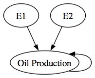
All this still begs the question of what is the best predictor of US retail sales. My approach is different from other forecasts that rely on models. Rather than advancing one model based on some argument, I test multiple models and choose the best one based on the AIC criterion: the best model is the one that predicts the historical data best with the fewest parameters. In this case, I tested the following models: (1) a random walk, R(t) = R(t-1) + E where R is Retail Sales and E is error, (2) a business-as-usual model, R(t) = a R(t-1) + E, (3) a state space model of the US economy, R(t) = a R(t-1) + S(US) + E where S(US) is the state of the US economy and (4) a state space model of the world economy,  R(t) = a R(t-1) + S(W) + E where S(W) is the state of the World economy. The states of the US and World economy are generated by the USL20 and WL20 models, respectively.

The rationale for these models is pretty straight forward: (1) given the high variability of the data, next year's sales may well be dominated by random error (the random walk), (2) if we smooth out some of the seasonal variability, average sales might just be a little bigger this year than last year (business-as-usual), (3) more realistically, US retail sales might depend on the entire state of the US economy and (4) given the globalization of world trade in retail services, the state of the world economy may be a better predictor of US sales.

The winner of the AIC competition was in fact the World economy model. The forecast with 98% prediction intervals from 2007-2015 is presented above. The best performance for retail sales was in 2007 and 2008. The worst performance was in 2009 and the first months of 2010. The sector has now pretty much recovered along with growth in the World economy. Returning to the FFC forecast of US retail sales growth rates, the forecast predicts an average annualized yearly growth rate of 2.07% for the period 2012-2015, very close to the current FFC number.

We've come a long way from the idea that Black Friday Retail Sales might be considered a reasonable predictor for yearly retail sales and learned that the US Retail Sector is part of the World economy. We've also learned that end-of-year sales are improbably (outside the 98% prediction interval) important to the sector. And, we've learned that setting up a single model to test a false problem is not a particularly useful way to conduct research.

TECHNICAL NOTE: The RSAFSNA.model is available here. Instructions for using forecasting models are available here. Once you have the R program installed and the dse, matlab, and scatterplot3d packages installed, you can run the following commands from the R console to display how well the best RSAFSNA.model fits the data.

> W <- "Absolute path for location of ws procedures"

> setwd(W)

> source("LibraryLoad.R")

> load(file="WL20v3_model")

> load(file="ws_procedures")

> 

> W <- "Absolute path for RSAFSNA model"

> setwd(W)

> load(file="US_RSAFSNA_model")

> m <- getModel(RSAFSNA.model,type="world index")

> tfplot(m)

You will notice that the model does not track the month-to-month variability in RSAFSNA. If we wanted to better predict things like end-of-year sales bumps, we could use seasonal dummy variables coded for the months of interest, for example November and December.

If you are interested in how the other models did, enter

> tfplot(m1 <- getModel(RSAFSNA.model,type="rw"))

> tfplot(m2 <- getModel(RSAFSNA.model,type="us index")) 

> tfplot(m3 <- getModel(RSAFSNA.model,type="bau"))

The plots actually seem to do a little better job of tracking the month-to-month variability. However, the AIC still suggests that the world model is best, but not by a huge amount.

> z <- bestTSestModel(list(m,m1,m2,m3))

Criterion value for all models based on data starting in period:  10 

5301.765 5354.228 5318.493 5377.438 

If you want to see the entire forecast with 98% bootstrap confidence intervals, enter

> b <- getModel(RSAFSNA.model,type="boot forecast")

> tfplot(b,m)

A More Conservative Peak Oil Forecast

In an earlier post (here) I presented a Peak Oil forecast that was pretty pessimistic: world oil production would collapse by 2040. I have been reluctant to publish this forecast because (1) the conclusions seemed pretty catastrophic and (2) the prediction intervals just looked too good, that is, too narrow implying a high degree of confidence that I didn't have. Above is another Peak Oil forecast with different prediction intervals that seem more realistic, that is, the downturn in world oil production might persist for a while but there is some probability (however small) that new technologies will come along that allow oil production to continue expanding. 

The problem with the original set of prediction intervals is that they did not take into account the error in the WL20 state variables that were used as input variables to the Peak Oil forecast. It was simply assumed that the raw forecast outputs of the WL20 model were the best future predictors for the world system. In any conventional forecasting model that has input variables, it is typically assumed that the forecast input variables are the best future predictors for the system. The assumption is certainly questionable and, at minimum, does not recognize that any model-based forecast has uncertainty attached to its outputs. Here's a simple causal diagram:

Typically, forecasts only take E2 into account when construction a forecast as was done with my initial Peak Oil forecast. E1 is simply ignored even though there is clearly cascading uncertainty in the model.

The conservative forecast above essentially takes both the E1 and E2 errors into account when computing prediction intervals for oil production since E1 is transmitted indirectly through the WL20 state variables.

A question at this point would be what if we ignored the E1 path entirely and just predict Oil Production without any input variables, what I would call a business as usual or BAU forecast. The Hubbert curve or Hubbert peak models were essentially BAU models with a different functional form i.e., the Logistic Distribution Curve. The advantage of the BAU models is that there is no cascading uncertainty. The BAU forecast in the graph above predicts that oil production will approach a peak somewhere between 80 million and 140 million tons of oil equivalent and stay there forever. This forecast is probably consistent with the improbable upper prediction interval of our initial conservative forecast.

Aside from the fact that we know oil is a nonrenewable resource, why should we prefer any of these plausible forecasts over any of the others? If we limit ourselves to the step-ahead AIC criteria, the BAU model is the winner with [264.70 < AIC=240.18 < 309.53] compared to the world system model with [290.42< AIC=279.72 <315.11]. However, if instead we calculate the attractor-based AIC, the WL20 model is best with AIC = 278.58 as compared to AIC=538.30 for the random walk model and AIC=315.06 for the BAU model. In other words, the BAU model is good at predicting next year's oil production but not very good at looking 50 years into the future (recall that the attractor simulation starts in 1950 and, from that initial position, simulates oil production out to 2008).

My experience has been that single equation models such as the BAU model or the Logistic model, are good at step-ahead predictions and are not subject to cascading uncertainty from input variables. However, single-equation models are not necessarily very good at predicting into the future even if the confidence intervals look quite narrow. And, because attractor models describe a path the system wants to move toward, their predictions also make more theoretical sense. The key here is to run the attractor simulation and compare the AICs for that simulation rather than the step-ahead simulation.

The ultimate test of all this is to compare the actual path of oil production over the next thirty years to the predictions of the various models--I just won't be around to make that comparison. In the next post, I'll explain how to generate these forecasts for the next generation in case they are interested.

Using Forecasting Models

In an earlier post (here) I explained how to use the WL20 model and the ws (world system) package. In this post, I will explain how to use forecasting models such as the one used to make my Peak Oil forecast (here).

Assuming that you have followed my earlier post, have R installed on your machine and have also installed the dse and the matlab packages successfully, the forecasting models are all available here. For this demonstration, download the PeakOilIndexModel to your working directory. Then you can enter the following commands at the > prompt in the R console:

> W <- "the complete path name for your working directory"

> setwd(W)

> source(file="LibraryLoad.R)

> load(file="WL20v3_model")

> load(file="ws_procedures")

> load(file="PeakOilIndexModel")

The available forecasting models can be seen by typing (a help file for all the ws package functions is available here):

> summary(OIL.model)

The resulting listing will show each of the available models. For example,

[1] "BAU"

Eigenvalues of system matrix

[1] 0.9836614

[1] TRUE

     Parameter     Mean Mean LCI Mean UCI P>=T[1] P< T[1]

[1,]  240.1784 288.4285 264.6985 309.5271       1       0

     Std. Dev.      Bias    Bias-z

[1,]  18.21428 -48.25009 -2.649025

attr(,"class")

[1] "boot"

[1] "STRUCTURAL"

NULL

The BAU (Business As Usual) entry shows a number of statistics used to evaluate the model. The Structural model displays NULL because no structural model was estimated.

The first statistic displayed for the BAU model is the eigenvalue of the system matrix. If all the eigenvalues are less than unity, the model is stable, which is displayed next as [1] TRUE. The next line shows the bootstrap distribution of the AIC statistic. The first value, 240.1784, is the sample AIC statistic. The second value is the bootstrap mean AIC statistic. The third and fourth values are the lower and upper 98% confidence intervals for the AIC statistic. The remaining values display probabilities, standard deviation and bias for the sample AIC statistic. If you want to inspect the BAU model, enter:

> getModel(OIL.model,type="bau")

Given the AIC statistics, the BAU model is the best one observed. For the forecast, however, I used the  best attractor model which you can display with

> getModel(OIL.model,type="best attractor")

The best attractor model is based on a free-simulation of each estimated model and is chosen using the AIC statistic from the free simulations vs. the actual data residuals. In this case, the world index model

> getModel(OIL.model,type="world index")

provides the best attractor simulation. You can get a flavor for the differences in the predictions from the two models by entering:

> tfplot(sim(getModel(OIL.model,type="bau")))

> tfplot(sim(getModel(OIL.model,type="world index"),sampleT=95,input=WL20.fx))

The BAU model predicts a gradual decline over time in the rate of oil production while the best attractor model shows a sharp peak-and-collapse between 2000 and 2020. 

Why should we be willing to choose one of these models over the other? One is best by conventional standards (step-ahead predictions using the AIC). Another is best by standards derived from attractor theory and application of the AIC criteria to the free simulations of each model. 

In future posts, I'll work through this issue and also reveal some more of the things you can do with the forecasting models using the dse and the ws packages. At this point, you should be able to at least load and inspect the models.

Peak Oil Forecast and Global Warming

Peak Oil is the point where the rate of petroleum extraction starts declining because the resource is being exhausted.  US domestic Peak Oil production was reached in 1970. World oil production may have peaked in 2011, but it is too early to establish that as fact. In this post, I will forecast World oil production using the WL20 model to see whether the model thinks the World system has reached Peak Oil.

If you've "peaked" at the graphic above you probably can determine that the answer will be "Yes"! However, there's much more at stake here than the simple conclusion, however controversial, that we have reached Peak Oil.

After seeing my Global Warming forecast (here), one of my readers wondered whether anyone had combined Peak Oil models and Global Warming models. He reasoned, correctly, that the  WL20 model was capable of exploring the link between Peak Oil and Global Warming. This post will explore that relationship.

The underlying theoretical model linking Peak Oil and Global Warming is pretty simple: (Oil Production) -> (CO2 Emissions) -> (Global Warming). You might disagree with this linear causal model, but assume for the moment that it is correct. Then, anything that reduces oil production, like Peak Oil, will reduce Global Warming. My Global Warming forecast (here) shows Global temperature peaking sometime between 2040 and 2060. My Peak Oil Forecast above shows that oil production has reached its peak and is likely to collapse entirely around 2040. The result would seem to confirm the simple theoretical model, but how are these two forecasts related within the WL20 model?

The WL20 model model is a state-space model with three state variables (these state variables were not imposed on the model a priori but were the result of the statistical analysis): the first state variable measures overall growth in the World system; the second state variable measures declining biodiversity; and, the third state variable measures increasing resource constraints in the commodity markets related to the Ecological Footprint. The three state variables are interrelated: increasing biodiversity is related to declining global temperature while  increased resource extraction through commodity markets and overall economic growth are related to positive increases in global temperature.

The early peak in oil production is just one of a number of negative feedback loops within the model. The negative feedback loops limit overall growth in the World system around 2040 (see the WL20 state-variable forecast here). Global temperature takes a few more decades to peak after that, but it is really the end of overall growth, not just Peak Oil, that eventually limits global temperature growth, at least in the WL20 model.

There seem to be very few studies that have pursued the link between Peak Oil and Global Warming possibly because there are many alternative, high-carbon sources of energy (tar sands and synfuel from coal being two examples) that could be substituted for oil. Others, such as Amory Lovins (here) have argued that "Efficiency is cheaper than fuel" and will, for economic reasons, eventually limit emissions along with cheaper green energy. The WL20 model is capable of making projections of economic efficiency, a topic I will have to return to in a future post. The difficulty with the "substitution" argument is the important extent to which the entire World system is built on the oil economy. Even though we switched from a coal- to an oil-based economy in the 20th Century, it's not clear that the next energy conversion will be that easy given the larger scale of the present World system.

`

The prediction of Peak Oil was initially made by M. King Hubbert, a Shell geoscientist who died in 1989. The Hubbert curve or Hubbert peak for the World system is displayed above (from this source). His forecast, based on logistic curve modeling, predicted that the peak in World oil production would occur in the year 2000. It serves as a warning that no forecasting model can really see into the future. The models are simply attempts to explore the future implications of the data and models available when the forecast was made.

Using the WL20 Package

The WL20 (W stands for World and L20 stands for Late 20th Century) package is an aggregate, state-space model of the World system. It contains 14 variables thought to be important to measuring the state of the World system, to include population growth, urbanization, commodity markets, carbon emissions, global temperature, biodiversity, globalization and the Ecological Footprint.

Unlike other World models, such as the DICE model, the Wonderland Model, or the System Dynamics World Models, WL20 was not derived from purely theoretical considerations. Rather, it was based on a 1979 paper by R. E. Kalman titled A system-theoretic critique of dynamic economic models. In the paper, Kalman argues that, until complex social systems are better understood, it is important to work from

data -> model

rather than from first-principle, theoretical considerations. In this approach, the primary emphasis is the selection of the data to describe the system followed by the use of state-space models to describe the dynamic behavior of the system. There is some theory used to make the selection of data that I have already discussed (here) and will discuss more fully in a future post. This post will concentrate on the computing details of the model.

The WL20 state-space model was estimated using the dse package (here) and the matlab package (here) in the public domain (it's free) R statistical language (here). Documentation, procedures and the WL20 model are available here.  They should be downloaded to a directory on your computer with the absolute path described by W (see below). The remainder of this post describes how to use the WL20 model using the R statistical language.

When you start R on your computer, the R console window will display the version number, copyright information and platform. On my computer:

R version 2.14.2 (2012-02-29)

Copyright (C) 2012 The R Foundation for Statistical Computing

ISBN 3-900051-07-0

Platform: i386-apple-darwin9.8.0/i386 (32-bit)

A number of  commands that you might find useful will also be displayed

R is a collaborative project with many contributors.

Type 'contributors()' for more information and

'citation()' on how to cite R or R packages in publications.

Type 'demo()' for some demos, 'help()' for on-line help, or

'help.start()' for an HTML browser interface to help.

Type 'q()' to quit R.

To use the WL20 package,  the dse and matlab packages must also be installed (use the "Package Installer" menu choice and be sure to check the box marked "Install Dependencies" after you get the list of "CRAN (binaries)", you can then select matlab and dse and click "Install Selected"). You can then run R and enter the commands below in the R console window (the > is the R prompt). 

> W <- "a character string describing the working directory location"

> setwd(W)

> source("LibraryLoad.R")

> load(file="ws_procedures")

> load(file="WL20v3_model")

> WL20.est

The first two commands assign and set the working directory to the file folder where you have downloaded the WL20 package. For example, on my computer, W is set to:

> W <- "/Users/georgepa/Desktop/R/Papers/WL20 v3/"

The next command will source the dse and matlab packages (if you get error messages, these packages have not been installed properly). The two load commands load the ws (world system) procedures and the model (if you get error messages here, you have probably not specified W properly). The final command displays the state-space model matrices for the WL20 model. These matrices are defined in the dse documentation that you can display with the following command:

> help(SS)

Data for the WL20 model were gathered from a number of sources, but mostly from the Earth Policy Institute's Data Highlights (here). The complete list of the data sources is available in the documentation (Appendix F, here). You can look at the first few lines of the data set using the following commands:

> head(WL20.data)

          N   OIL  QA GWP P.Wheat. P.Oil.  TEMP   CO2 Carbon

[1,] 2555.0 10.42 631 7.4     1.89   1.71 13.83 311.3   1630

[2,] 2597.5 11.73 655 7.9     2.03   1.71 13.98 311.7   1767

[3,] 2641.2 12.34 680 8.3     1.93   1.92 14.04 312.2   1795

[4,] 2686.2 13.15 705 8.6     1.89   2.01 14.12 312.7   1841

[5,] 2732.5 13.74 730 8.9     1.98   2.11 13.91 313.2   1865

[6,] 2780.0 15.41 759 9.4     1.81   2.11 13.92 313.7   2043

     TotalFootprint    Earths WorldGlobal LivingPlanet    URBAN

[1,]       5.292910 0.4597521    23.37150     1.000000 705.4807

[2,]       5.493554 0.4797747    23.94942     1.002878 730.5622

[3,]       5.694199 0.4997972    24.52735     1.005581 756.4242

[4,]       5.894843 0.5198197    25.10527     1.007935 783.1143

[5,]       6.095488 0.5398423    25.68320     1.009766 810.6524

[6,]       6.296133 0.5598648    26.26112     1.010900 839.0286

The data set runs from 1950 to 2008, which you can verify with the following commands:

> start(WL20.data)

[1] 1950    1

> end(WL20.data)

[1] 2008    1

There are commands in the dse package that you can use to evaluate this model. For example:

> roots(WL20.est)

[1] 1.0000000+0.000000i 0.9982313+0.027957i 0.9982313-0.027957i

[4] 0.9140820+0.000000i

attr(,"class")

[1] "roots"

displays the eigenvalues of the system matrix. The first eigenvalue (1.0000000+0.000000i) is unity because the model includes a constant. The other eigenvalues are all less than unity and have imaginary parts indicating that the model is stable but cyclical.

You can also check the model fit using:

> tfplot(WL20.est)

The results are displayed above. The dotted line displays the fitted values (one step ahead predictions) and the solid lines display the actual state variables.

The WL20 model has three state variables labelled W1, W2 and W3 in the graphic above. The state variables were constructed using Principal Components Analysis (PCA). The measurement model from the PCA is displayed with the following command:

> measurementModel(WL20.index)

               N        OIL          QA         GWP  P.Wheat.

[1,]  0.28446020  0.2711239  0.28207253  0.28243781 0.2362789

[2,] -0.01609311  0.2410390  0.09853503 -0.14131911 0.4113772

[3,] -0.11117409 -0.2412009 -0.08825703  0.02134276 0.4610974

         P.Oil.       TEMP         CO2      Carbon TotalFootprint

[1,] 0.24295530  0.2514421  0.28373276  0.28328608      0.2752374

[2,] 0.06595202 -0.2352280 -0.09832577  0.09252815      0.1816798

[3,] 0.71181845  0.1901141 -0.02009544 -0.09553557     -0.2925719

         Earths WorldGlobal LivingPlanet       URBAN

[1,]  0.2787654  0.28189899  -0.18387870  0.28400812

[2,]  0.1484351 -0.09256627   0.77050207 -0.08681005

[3,] -0.2311710 -0.09431697  -0.05760175 -0.07067596

The rows of this matrix display the weights used to calculate W1, W2 and W3. The weights were constructed from standard scores of the input data. The weight attached to each indicator variable for each state variable are displayed in the columns. By construction, the state variables are independent and uncorrelated.

The pattern of the weights indicated that W1 measures overall secular growth in the World system (this can also be seen from the time plot of W1 above). The second measure is most heavily weighted on the Living Planet Index (0.77050207), wheat prices (0.4113772), oil production (0.2410390) and the Ecological Footprint (number of Earths used by the World System, 0.1484351). The W2 state variable thus measures biodiversity. Finally, the W3 state variable is weighted most heavily on oil prices (0.71181845), wheat prices (0.4610974), Total Ecological Footprint (-0.2925719), and oil production (-0.2412009). The W3 state variable thus measures the effect of commodity markets and the Ecological Footprint.

> WL20.index$measurement$output$fraction.variance

 [1] 0.8740847 0.9413934 0.9725388 0.9864508 0.9949011 0.9980068

 [7] 0.9987371 0.9993400 0.9997902 0.9999405 0.9999802 0.9999923

[13] 0.9999986 1.0000000

Taken together, the World system state variables explain 97% of the variation in the underlying indicators.

One important use of the WL20 model is to forecast future states of the World system. The following commands create and display a 100 year forecast of the state variables:

> f <- forecast(WL20.est,horizon=100)

> tfplot(f)

The results of the forecast, displayed above, indicate that growth in the World system is expected to peak between 2040 and 2050 (W1)  associated with continuing losses of biodiversity (W2) and increasing pressure on commodity markets (W3). You can obtain the entire forecast to use as input to there times series models with the following command:

> fx <- merge.forecast(f)

The WL20 forecast and the time series are already available to you as data files named WL20.f and WL20.fx, respectively. 

I have already used forecasts from the WL20 model to predict global climate change and other indicators (here and here). In future posts, I will make the forecasting models models available as state-space models that can also be loaded into your R workspace and run on your machine.

TECHNICAL NOTE: In the Kalman article (here), emphasis is placed on the importance of observability and controllability in the selection of state space models. For the WL20, these two features can be checked with the following commands:

> observability(WL20.est)

[1] 2.5510918 2.2200285 1.8375940 0.6061376

> reachability(WL20.est)

Singular values of reachability matrix for noise:  2.424642 2.20612 1.628193 1.202821e-16 

The commands display the singular values of certain state-space matrices (use help for more information). If all the singular values are greater than zero, the model is both observable and controllable. The WL20 model is completely observable but might not be totally controllable (the 1.202821e-16 principal value is effectively zero). 

US Real GDP Growth in 2012

The Financial Forecast Center (FFC here) produces a forecast for US nominal GDP. From the graphic above, FFC is expecting little growth in the first two quarters of 2012. FFC presents two confidence bands for each value. For example, in Jan 2012, FFC is forecasting nominal GDP at $15,333B. The 50% correct band would be +/- 112 while the 80% correct band would be +/- 225. The bands get bigger over time as expected but the GDP value stays at $15,433B through June of 2012, the end of the FFC forecast period.
I would prefer to forecast real GDP since it would not be clear for a nominal GDP forecast how much trends would be affected simply by prices (the GDP deflator). I would also rather forecast the attractor value since we are just coming out of the Subprime Mortgage Bubble and Collapse.

My attractor forecast for real GDP taken from the BEA (here) is presented in the graphic above. The bubble and collapse is clearly displayed. Currently we are at the lower 98% prediction interval for the attractor. This suggests that GDP will be drawn higher in 2012 (a return to the attractor value) unless other events (such as the EU sovereign debt crisis) continue to weight down the US economy (the mechanism of transmission here could be either a reduction in US exports to the EU or more financial contagion).

The FFC does produce a US Real GDP growth rate forecast (here and in the graphic above). The FFC is predicting a reduction in real GDP growth down to around 0.6% in the second quarter on 2012 (50% +/- 1.1% and 80% correct +/-2.4%).

My average annualized growth rate forecast for 2012 is 1.5% which is close to the FFC forecast of 1.6% for the first quarter of 2012. The FFC forecast of 0.5% growth in the second quarter of 2012 is possible but not that likely since the economy is not on its attractor value in the first quarter of 2010.

As a comparison, my mean annualized attractor growth rate for the period 2004-2007 was 1.6% while the actual mean annualized growth rate was 2.5%, 1 full point being attributable to the bubble.

NOTE: The attractor value results from a free simulation of GDPC96 starting in 1960 being driven by the state variables from the WL20 model. The WL20 model produces the best attractor as determined by the AIC criterion. A typical forecast predicts from year to year. The prior year contains shock and bubble values that bias the forecast.