Calculating Forecasting Odds: Think Like a Stockbroker

In a Take Part article (here), Amy Luers, Director of Climate Change at the Skoll Global Threats Fund, takes on the issue of variability and forecasting. Leurs makes the argument that global temperature forecasting and stock forecasting have similar problems with statistical variability. Working with Leonard Sklar, Professor of Geology at San Francisco State University, Leurs developed the two graphs above. On the left is the Dow Jones Industrial Average (DJI, my forecast for the SP500 is here), on the right is Global Temperature (my forecast is here). The bottom left graph shows the odds of making money if you invested in any random year (1913-2010) and stayed in the stock market for up to 50 years. After about 35 years of staying invested, there is a 100% chance of making money. On the right is the same graph for global temperature. It takes a little longer, but after 45 years you have a 100% chance of finding a temperature increase. Notice that in both cases, if you look over only brief periods, the odds are closer to 50-50.

The graph above is from page 381 of Nate Silver's book The Signal and the Noise. In 2007, the notorious Scott Armstrong, Professor of Marketing at the Wharton Business School, made a $10,000 bet with Al Gore that Armstrong modestly called "The Global Warming Challenge." Armstrong and his colleague Kesten Green, an Australian Business School Lecturer,  have argued (here) that Global Temperature is too variable to forecast. The Armstrong-Gore bet was to be resolved monthly. Predicting "no-change," Armstrong argued from the data above that he had won the bet.

Given the Luers-Sklar data, we understand why Armstrong made this bet and we also understand why Al Gore never took the bet. Five years is far too short a time to determine whether temperature has increased or whether, for that matter, the stock market has made money. Having published "Principles of Forecasting, [...a book that...] should be considered canonical to anybody who is seriously interested in the field [...of forecasting]" (these are Silver's words), Prof. Armstrong should have known better.

The basic problem with Prof. Armstrong, his "Global Warming Challenge" and his forecasting principles (I have commented on the principles here) is summed up by a quote from Nelson Mandela "Where you stand depends on where you sit" and Prof. Armstrong sits in the business school and is paid to market business activity as having little impact on the environment. All the forecasting principles and outrageous bets in the world will not cover up this canonical conflict.

The Mystery of Why Portugal's Economy Has Performed So Poorly.

Portugal's Economy is Heading for a Steady-State

Oct 22, 2026 Cost of living protests hit Belgium, Italy, Portugal and France Hundreds of thousands of Europeans have taken to the streets in separate, uncoordinated demonstrations to protest against the rising cost of living in their countries.

Matthew O'Brien recently wrote a piece for the Atlantic titled "The Mystery of Why Portugal Is Doomed". The reasons given in the piece are all essentially recitals of the conventional wisdom on economic development and, although each point might make sense in and of itself, the actual causes are simpler to understand and less complicated. From the graph above (real GDP in US$ from the World Data Bank) the economy in Portugal experienced an economic bubble after it joined the EU in 1999 and the bubble popped in 2007 as a result of the Subprime Mortgage Crisis. The bubble can be clearly seen in the dynamic attractor plot above (the dashed red line is the dynamic attractor path and the other dashed lines are the 98% bootstrap prediction intervals). Before going into more detail, let's review the conventional wisdom.

Matthew O'Brien lists the following problems with the economy of Portugal:

• Between 2000 and 2012, Portugal's economy wasn't growing fast enough. To prove this case, GDP per capita in Portugal from 2000-12 is compared to the USA 1929-41 (the Great Depression) and Japan 1992-2004 (the Lost Decade). The comparison supposedly supports the conclusion that "this wasn't the case of the bust erasing the boom, because there was no boom". But this is certainly a logical non-sequitur since these economies and time periods really have nothing to do with each other (more about the supposed "non-boom" and a-historical comparisons later).
• Portugal's Immature Financial Sector. After Portugal's entry into the EU, the financial sector "...misallocated the foreign capital that poured in to low productivity, non-tradeable sectors like wholesale and retail trade. In other words, it wasted money on things that never had a chance of paying off." This argument is rejected because German Banks in Portugal also made "bad bets". Bankers making bad bets sounds consistent with bubble behavior which seems inconsistent with the "non-boom".
• Portugal's Small Business Culture, Too Much Corruption and Regulation. Portugal and all of Southern Europe supposedly have too many small "mom-and-pop" businesses that stay small to fly under the radar of a corrupt government. The conventional wisdom: if small-and-medium-sized-enterprises (SMEs) play too big a role in the economy, the economy can't grow and take advantage of economies of scale. The article correctly rejects this explanation because it has been true for most of the late 20th century and hasn't changed much recently.
• Portugal Has To Fix All The Structural Problems.  Here the article trots out the laundry list of conventional criticism of Southern European countries: labor market inflexibility (they need to fire more workers), difficulty starting a business (too much red tape), and legal problems (inability to enforce contracts). "After all, Portugal's stagnation between 2000 and 2008 shows that adequate demand isn't sufficient in the face of these deep problems--but it is necessary. That's why Europe needs to stop insisting on punishment as the path the prosperity." What seems more interesting about the period after 2000 when looking at the graph above is why the bubble was able to stay inflated for so long?

In the end, the article concludes that Portugal's economic performance is a "puzzle". What creates the puzzle, I would argue, is illogical comparisons and arbitrary lines (explicitly or implicitly) drawn on graphs.

The starting point for all the consternation about Portugal is the counterfactual assertion that Portugal should have grown more rapidly. The counterfactual assertions can be conveniently summarized by drawing lines on graphs (the solid red lines with arrows in the graph above) projecting rapid future growth based on strong periods of (bubble driven?) economic performance.  Portugal should have taken-off after the mid-1990s (Dot-com bubble), or after 1999 (EU bubble, "I contend that the European Union itself is like a bubble." George Soros, June 2, 2012) or after 2007 (Subprime Mortgage Housing bubble). Something must have been preventing the take-off into sustained growth implied by the red-line counterfactuals and the usual culprits are trotted out to affirm the conclusion.

None of the red-line "take-off" extrapolations have anything to do with the capabilities of Portugal's economy but rather with the implications of neoclassical economic growth models. Unfortunately, Portugal's economy is not correctly described by the unrestrained exponential growth embedded in such models. Portugal's growth is slowing because the economy is moving toward a steady state. To understand these issues, which are very different from the conventional wisdom, will require a comparison of the neoclassical growth model to the PT20 state-space model of Portugal's economy (the model used to generate the dynamic attractor path in the plot above) and a more detailed discussion of macroeconomic analysis underlying the conventional wisdom, to be covered in future posts.

The Sequestration Experiment: Forecast, Counterfactual or Muddle?

On March 1, 2013 President Obama signed the executive order that put the 2013 Sequestration into effect. Budget Sequestration, first used in the  Gramm-Rudman-Hollings Deficit Reduction Act of 1985 (GRHDRA), places an automatic spending cap on the federal budget. If Congress exceeds the cap through spending authorizations (remember, Congress authorizes spending in the US Government) automatic cuts take place. The total size of the 2013 Sequestration is $85.4 Billion.

From Keynesian Economics 101 we all know that Y = I + C + (X-M) + G, that is, national income is composed of expenditures on investment (I), consumption (C), the balance of trade (Exports - Imports, X-M) and government expenditure (G). Everything else being equal, a cut in G will reduce Y. Therefore, the 2013 Sequestration should result in a recession, that is, a drop in overall national income.

In the graph above, produced by Macroeconomic Advisers (a nonpartisan organization that uses a complex macroeconomic model of the US economy to generate forecasts), the annual percentage change in real GDP (think National Income divided by the aggregate price level) with and without Sequestration is displayed. The blue line shows that Sequestration knocks a few percentage points off real GDP growth for all of 2013 but afterward there is no lasting impact compared to the gradual reductions in government spending assumed in the baseline (the red line).

Essentially the graph shows that Sequestration (really, enforced Austerity) inflicts unnecessary hardship on everyone affected by it from the Defense Department to poor children in Head Start. This is an important point but it misses the bigger picture. The Right Wing has been arguing ever since the Great Depression in the 1930s that Austerity (cutting government expenditure) is the correct response to Depressions and Recessions. Their argument is that since government gets its income from taxation, any reduction in taxation will put money in everyone's pockets to be used to pull the country out of Recession. If the government spends through borrowing, the spending is taking money away from investment (I) so there will be no effects on national income (Y). If government spends by printing money this will create inflation and have no impact on real GDP.

There are many arguments that can and have been made against this reasoning (you can read these arguments in economist Paul Krugman's blog on the NY Times here). Let's assume for the moment that  each position (Keynes vs. the Classics) is just a theory. Testing these two theories is not easy because it would require a macroeconomic experiment that no economist can run. I cannot simply cut aggregate government expenditure and see what happens. I can develop a model of the economy (such as the one developed by Macroeconomic Advisers), include government expenditure as an input variable, cut the level of this input variable holding everything else constant and see what happens. But, I am working with a model not the real economy and the model is subject to specification error.

In the $85.4 Billion 2013 Sequestration, however, we have a perfect natural experiment. Now we will finally get an answer to the major macroeconomic debate of the last 100 years. Unfortunately, we will not get this answer because political forces are working to muddle the experiment. The House GOP promises to limit the effects of Sequestration on Defense, Law Enforcement and Border Patrol. The old arguments about big government and excessive spending get put aside when arguably the most wasteful part of government, the Defensed Department, is facing cuts.

In what different Universe would we just run the experiment and settle the question once and for all? In the end, all that will remain is our ability to run counterfactual experiments with our models, experiments no one seems willing to accept.

Looking Back on 2011-2012 Fictions

This blog is based (somewhat) on a book by Nelson Goodman titled Fact, Fiction and Forecast (click the link to read a free pdf copy of the Fourth Edition). Goodman argued (summarized here) that Facts (things we observe from past history) and Fictions (counterfactuals) are more difficult to form into law-like statements that we can use to make Forecasts (predictions about the future) than we might think. My reaction to reading the initial edition in the 1980's was all these issue are related to building mathematical models. A mathematical-statistical model estimated from data (facts) can be used to generate counterfactuals by change some of the model parameters and also used to make forecasts by running the models into the future. The quality of a model will depend on its ability to do these things and, rather than arguing about formal aspects of the model, we need to get on with the enterprise and see how well models perform.

Surprisingly or not, in the social sciences this isn't really done with much enthusiasm. Models are estimated, journal articles are published or policy recommendations made, and the performance of the models is rarely critiqued over time. This state of affairs became a problem in the Economics profession during the Subprime Mortgage Crisis (for example, the Federal Reserve econometric models were "wildly inaccurate"). Why hadn't complex econometric models seen the crisis coming? And, if they had, why weren't alarms raised? For example, econometric models of mortgage default risk were found to be unstable and basically useless in predicting future mortgage defaults (here). And, Early Warning System (EWS) models, based on standard indicators, "...frequently do not provide much advance warning of currency and banking crises" (here). I discussed the forecasting problem in an early post (here).

Since I have been developing macro-societal statistical models since the late 1970's and have not really followed up much in my career on how well the models were performing, I thought now we be a good time to get on with it. I have about two years worth of experience looking at how well state-space time series models perform when estimated from historical data (facts), how well the same models can be used to generate counterfactuals (What if the US had increased levels of deficit spending? Would the crisis have been of shorter duration?) and how well the model forecasts have compared to those of other forecasters (particularly the Financial Forecasting Center which uses Artificial Intelligence models).

My first attempt at a counterfactual using the USL20 model was in September of 2011 (here). The Obama administration was essentially making the argument that without the bailout of the financial system, the US economy would have "gone off the cliff" after 2009 (when the Obama administration came into office). They way I constructed this counterfactual was to estimate the state space model up to 2008, the end of the Bush administration, and then run model forward as if the Bush administration had stayed in power and the Obama administration policies had never been enacted. In other words, forecast forward from 2008 to 2011 without knowledge of what actually happened. The economy (GDP in this case) should have gone off the cliff. It didn't. In fact, the economy actually performed a little better in the counterfactual world (dotted red line in the graphic above) than in the real world (solid black line).

Now, there were lots of reasons why the economy did not perform very well in the later part of 2011, the Sovereign Debt Crisis in Europe for one, in addition to the policies of the administration in power. But one thing the counterfactual did demonstrate was that the stimulus was not a "tremendous success" as was being argued by Time magazine (here).

There is a lot more counterfactual work that needs to be done surrounding fiscal policy and monetary policy in response to the US Subprime Mortgage Crisis. The counterfactual above suggests a pretty limited role for fiscal and monetary policy once a bubble pops (more work at different times in different countries needs to be done to demonstrate this point). If this assertion is confirmed, it still doesn't mean that policy measures might not have prevented the bubble from developing in the first place. The counterfactual would be to find some set of policy measures that would prevent the Housing and Stock Market Bubbles. Again, more work would have to be done at different time points and in different countries. And, we need better ways of identifying bubbles while they are developing (this is the topic of another blog here).

US Retail Sales

Retail sales became the object of controversy this year when Paul Dales of Capital Economics challenged the "conventional wisdom" that Black Friday sales are a good predictor of yearly sales. In other places (here and here) I've described how the methodology used by Mr. Dales is probably flawed (I actually don't know what methodology was used but I made some guesses based on computer simulation). Another questionable part of Mr. Dale's work is the idea that any week during the year would be a good predictor of yearly sales. Sales forecasts would typically be based on some type of macro-economic time series model that uses multiyear data, the more the better. In this post, I will use multiple state space models to predict US retail sales. The results suggest a different story about what drives yearly sales in the US retail sector.

The Financial Forecast Center generates forecasts of US Retail Sales Growth Rates (here). The current forecast is displayed in the graphic above. The forecasts are generated with artificial intelligence software, not macro-economic models. As such, the FFC models do not have the biases associated with models based on a priori theoretical considerations. Their results show that retail sales growth rates have been declining since 2010 and are predicted to drop below 2% by 2013.

The FFC provides monthly, not seasonally adjusted, retail sales data (RSAFSNA) taken from the US Department of Commerce (here) in millions of dollars starting in 1992. When we plot that data for the period 2007-2012 (from the beginning of the financial crisis to the beginning of this year) we see very clearly that retail sales are elevated during the last two months of each year and that peak year-end sales pretty much follow trends for the rest of the year. The graph alone refutes the idea that Black Friday is a bunch of meaningless hype.

All this still begs the question of what is the best predictor of US retail sales. My approach is different from other forecasts that rely on models. Rather than advancing one model based on some argument, I test multiple models and choose the best one based on the AIC criterion: the best model is the one that predicts the historical data best with the fewest parameters. In this case, I tested the following models: (1) a random walk, R(t) = R(t-1) + E where R is Retail Sales and E is error, (2) a business-as-usual model, R(t) = a R(t-1) + E, (3) a state space model of the US economy, R(t) = a R(t-1) + S(US) + E where S(US) is the state of the US economy and (4) a state space model of the world economy,  R(t) = a R(t-1) + S(W) + E where S(W) is the state of the World economy. The states of the US and World economy are generated by the USL20 and WL20 models, respectively.

The rationale for these models is pretty straight forward: (1) given the high variability of the data, next year's sales may well be dominated by random error (the random walk), (2) if we smooth out some of the seasonal variability, average sales might just be a little bigger this year than last year (business-as-usual), (3) more realistically, US retail sales might depend on the entire state of the US economy and (4) given the globalization of world trade in retail services, the state of the world economy may be a better predictor of US sales.

The winner of the AIC competition was in fact the World economy model. The forecast with 98% prediction intervals from 2007-2015 is presented above. The best performance for retail sales was in 2007 and 2008. The worst performance was in 2009 and the first months of 2010. The sector has now pretty much recovered along with growth in the World economy. Returning to the FFC forecast of US retail sales growth rates, the forecast predicts an average annualized yearly growth rate of 2.07% for the period 2012-2015, very close to the current FFC number.

We've come a long way from the idea that Black Friday Retail Sales might be considered a reasonable predictor for yearly retail sales and learned that the US Retail Sector is part of the World economy. We've also learned that end-of-year sales are improbably (outside the 98% prediction interval) important to the sector. And, we've learned that setting up a single model to test a false problem is not a particularly useful way to conduct research.

TECHNICAL NOTE: The RSAFSNA.model is available here. Instructions for using forecasting models are available here. Once you have the R program installed and the dse, matlab, and scatterplot3d packages installed, you can run the following commands from the R console to display how well the best RSAFSNA.model fits the data.

> W <- "Absolute path for location of ws procedures"

> setwd(W)

> source("LibraryLoad.R")

> load(file="WL20v3_model")

> load(file="ws_procedures")

> 

> W <- "Absolute path for RSAFSNA model"

> setwd(W)

> load(file="US_RSAFSNA_model")

> m <- getModel(RSAFSNA.model,type="world index")

> tfplot(m)

You will notice that the model does not track the month-to-month variability in RSAFSNA. If we wanted to better predict things like end-of-year sales bumps, we could use seasonal dummy variables coded for the months of interest, for example November and December.

If you are interested in how the other models did, enter

> tfplot(m1 <- getModel(RSAFSNA.model,type="rw"))

> tfplot(m2 <- getModel(RSAFSNA.model,type="us index")) 

> tfplot(m3 <- getModel(RSAFSNA.model,type="bau"))

The plots actually seem to do a little better job of tracking the month-to-month variability. However, the AIC still suggests that the world model is best, but not by a huge amount.

> z <- bestTSestModel(list(m,m1,m2,m3))

Criterion value for all models based on data starting in period:  10 

5301.765 5354.228 5318.493 5377.438 

If you want to see the entire forecast with 98% bootstrap confidence intervals, enter

> b <- getModel(RSAFSNA.model,type="boot forecast")

> tfplot(b,m)

A More Conservative Peak Oil Forecast

In an earlier post (here) I presented a Peak Oil forecast that was pretty pessimistic: world oil production would collapse by 2040. I have been reluctant to publish this forecast because (1) the conclusions seemed pretty catastrophic and (2) the prediction intervals just looked too good, that is, too narrow implying a high degree of confidence that I didn't have. Above is another Peak Oil forecast with different prediction intervals that seem more realistic, that is, the downturn in world oil production might persist for a while but there is some probability (however small) that new technologies will come along that allow oil production to continue expanding. 

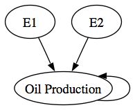
The problem with the original set of prediction intervals is that they did not take into account the error in the WL20 state variables that were used as input variables to the Peak Oil forecast. It was simply assumed that the raw forecast outputs of the WL20 model were the best future predictors for the world system. In any conventional forecasting model that has input variables, it is typically assumed that the forecast input variables are the best future predictors for the system. The assumption is certainly questionable and, at minimum, does not recognize that any model-based forecast has uncertainty attached to its outputs. Here's a simple causal diagram:

Typically, forecasts only take E2 into account when construction a forecast as was done with my initial Peak Oil forecast. E1 is simply ignored even though there is clearly cascading uncertainty in the model.

The conservative forecast above essentially takes both the E1 and E2 errors into account when computing prediction intervals for oil production since E1 is transmitted indirectly through the WL20 state variables.

A question at this point would be what if we ignored the E1 path entirely and just predict Oil Production without any input variables, what I would call a business as usual or BAU forecast. The Hubbert curve or Hubbert peak models were essentially BAU models with a different functional form i.e., the Logistic Distribution Curve. The advantage of the BAU models is that there is no cascading uncertainty. The BAU forecast in the graph above predicts that oil production will approach a peak somewhere between 80 million and 140 million tons of oil equivalent and stay there forever. This forecast is probably consistent with the improbable upper prediction interval of our initial conservative forecast.

Aside from the fact that we know oil is a nonrenewable resource, why should we prefer any of these plausible forecasts over any of the others? If we limit ourselves to the step-ahead AIC criteria, the BAU model is the winner with [264.70 < AIC=240.18 < 309.53] compared to the world system model with [290.42< AIC=279.72 <315.11]. However, if instead we calculate the attractor-based AIC, the WL20 model is best with AIC = 278.58 as compared to AIC=538.30 for the random walk model and AIC=315.06 for the BAU model. In other words, the BAU model is good at predicting next year's oil production but not very good at looking 50 years into the future (recall that the attractor simulation starts in 1950 and, from that initial position, simulates oil production out to 2008).

My experience has been that single equation models such as the BAU model or the Logistic model, are good at step-ahead predictions and are not subject to cascading uncertainty from input variables. However, single-equation models are not necessarily very good at predicting into the future even if the confidence intervals look quite narrow. And, because attractor models describe a path the system wants to move toward, their predictions also make more theoretical sense. The key here is to run the attractor simulation and compare the AICs for that simulation rather than the step-ahead simulation.

The ultimate test of all this is to compare the actual path of oil production over the next thirty years to the predictions of the various models--I just won't be around to make that comparison. In the next post, I'll explain how to generate these forecasts for the next generation in case they are interested.

Using Forecasting Models

In an earlier post (here) I explained how to use the WL20 model and the ws (world system) package. In this post, I will explain how to use forecasting models such as the one used to make my Peak Oil forecast (here).

Assuming that you have followed my earlier post, have R installed on your machine and have also installed the dse and the matlab packages successfully, the forecasting models are all available here. For this demonstration, download the PeakOilIndexModel to your working directory. Then you can enter the following commands at the > prompt in the R console:

> W <- "the complete path name for your working directory"

> setwd(W)

> source(file="LibraryLoad.R)

> load(file="WL20v3_model")

> load(file="ws_procedures")

> load(file="PeakOilIndexModel")

The available forecasting models can be seen by typing (a help file for all the ws package functions is available here):

> summary(OIL.model)

The resulting listing will show each of the available models. For example,

[1] "BAU"

Eigenvalues of system matrix

[1] 0.9836614

[1] TRUE

     Parameter     Mean Mean LCI Mean UCI P>=T[1] P< T[1]

[1,]  240.1784 288.4285 264.6985 309.5271       1       0

     Std. Dev.      Bias    Bias-z

[1,]  18.21428 -48.25009 -2.649025

attr(,"class")

[1] "boot"

[1] "STRUCTURAL"

NULL

The BAU (Business As Usual) entry shows a number of statistics used to evaluate the model. The Structural model displays NULL because no structural model was estimated.

The first statistic displayed for the BAU model is the eigenvalue of the system matrix. If all the eigenvalues are less than unity, the model is stable, which is displayed next as [1] TRUE. The next line shows the bootstrap distribution of the AIC statistic. The first value, 240.1784, is the sample AIC statistic. The second value is the bootstrap mean AIC statistic. The third and fourth values are the lower and upper 98% confidence intervals for the AIC statistic. The remaining values display probabilities, standard deviation and bias for the sample AIC statistic. If you want to inspect the BAU model, enter:

> getModel(OIL.model,type="bau")

Given the AIC statistics, the BAU model is the best one observed. For the forecast, however, I used the  best attractor model which you can display with

> getModel(OIL.model,type="best attractor")

The best attractor model is based on a free-simulation of each estimated model and is chosen using the AIC statistic from the free simulations vs. the actual data residuals. In this case, the world index model

> getModel(OIL.model,type="world index")

provides the best attractor simulation. You can get a flavor for the differences in the predictions from the two models by entering:

> tfplot(sim(getModel(OIL.model,type="bau")))

> tfplot(sim(getModel(OIL.model,type="world index"),sampleT=95,input=WL20.fx))

The BAU model predicts a gradual decline over time in the rate of oil production while the best attractor model shows a sharp peak-and-collapse between 2000 and 2020. 

Why should we be willing to choose one of these models over the other? One is best by conventional standards (step-ahead predictions using the AIC). Another is best by standards derived from attractor theory and application of the AIC criteria to the free simulations of each model. 

In future posts, I'll work through this issue and also reveal some more of the things you can do with the forecasting models using the dse and the ws packages. At this point, you should be able to at least load and inspect the models.