
In an earlier post (here) I presented a Peak Oil forecast that was pretty pessimistic: world oil production would collapse by 2040. I have been reluctant to publish this forecast because (1) the conclusions seemed pretty catastrophic and (2) the prediction intervals just looked too good, that is, too narrow implying a high degree of confidence that I didn't have. Above is another Peak Oil forecast with different prediction intervals that seem more realistic, that is, the downturn in world oil production might persist for a while but there is some probability (however small) that new technologies will come along that allow oil production to continue expanding.
The problem with the original set of prediction intervals is that they did not take into account the error in the WL20 state variables that were used as input variables to the Peak Oil forecast. It was simply assumed that the raw forecast outputs of the WL20 model were the best future predictors for the world system. In any conventional forecasting model that has input variables, it is typically assumed that the forecast input variables are the best future predictors for the system. The assumption is certainly questionable and, at minimum, does not recognize that any model-based forecast has uncertainty attached to its outputs. Here's a simple causal diagram:

Typically, forecasts only take E2 into account when construction a forecast as was done with my initial Peak Oil forecast. E1 is simply ignored even though there is clearly cascading uncertainty in the model.
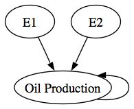
The conservative forecast above essentially takes both the E1 and E2 errors into account when computing prediction intervals for oil production since E1 is transmitted indirectly through the WL20 state variables.

A question at this point would be what if we ignored the E1 path entirely and just predict Oil Production without any input variables, what I would call a business as usual or BAU forecast. The Hubbert curve or Hubbert peak models were essentially BAU models with a different functional form i.e., the Logistic Distribution Curve. The advantage of the BAU models is that there is no cascading uncertainty. The BAU forecast in the graph above predicts that oil production will approach a peak somewhere between 80 million and 140 million tons of oil equivalent and stay there forever. This forecast is probably consistent with the improbable upper prediction interval of our initial conservative forecast.
Aside from the fact that we know oil is a nonrenewable resource, why should we prefer any of these plausible forecasts over any of the others? If we limit ourselves to the step-ahead AIC criteria, the BAU model is the winner with [264.70 < AIC=240.18 < 309.53] compared to the world system model with [290.42< AIC=279.72 <315.11]. However, if instead we calculate the attractor-based AIC, the WL20 model is best with AIC = 278.58 as compared to AIC=538.30 for the random walk model and AIC=315.06 for the BAU model. In other words, the BAU model is good at predicting next year's oil production but not very good at looking 50 years into the future (recall that the attractor simulation starts in 1950 and, from that initial position, simulates oil production out to 2008).
My experience has been that single equation models such as the BAU model or the Logistic model, are good at step-ahead predictions and are not subject to cascading uncertainty from input variables. However, single-equation models are not necessarily very good at predicting into the future even if the confidence intervals look quite narrow. And, because attractor models describe a path the system wants to move toward, their predictions also make more theoretical sense. The key here is to run the attractor simulation and compare the AICs for that simulation rather than the step-ahead simulation.
The ultimate test of all this is to compare the actual path of oil production over the next thirty years to the predictions of the various models--I just won't be around to make that comparison. In the next post, I'll explain how to generate these forecasts for the next generation in case they are interested.